Were the Ice Ages Caused by True Polar Wandering?
This is one of those things that once you see, you can’t un-see.
.
Table of Contents/Outline
Excerpts from my book, ‘Geophysics For The Coming Age: rewriting the modern geologic paradigm‘. (by Lance Weaver)
The following book brings together my three new theories and mechanisms for the evolution of the earth.
- My Galactic Double Interference Wave Theory (GDIW)
- My Precessional Polar Oscillation Cycle Theory (PPOC)
- My Core-Mantle Injection/Gas Exolution, Destabilization & Inflation Theory (CMIDI)
Given together, I dub them ‘Weaver TPW Oscillation Cycles’
These three theories work together to explain the earth’s tectonic and climatic cycles seen in ice cores, deep sea marine isotope data and the stratigraphic record and revise some of the prevailing views on plate tectonics, Milankovitch cycles, D-O events, our galaxy structure/formation, earth’s core-freezing dynamics and see-saw evidence as well as paleomagnetic data and extinction events.
It is a comprehensive model tying together much of the cutting edge research coming out of the massive amounts of data and visualizations gained over the last few decades. It posits that the earth goes through a galactically induced rapid TPW event about every ~3,000-12,000 years, caused by previously overlooked gravitational and electromagnetic forces associated with the earth’s well-known Milankovitch Cycles. In addition to causing earth’s precession cycles, these gravitational effects also slowly create volumetric mass imbalances (primarily from exsolved core gases) in the lower mantle boundary which then cause sudden realignments of the earth’s spin axis as our Solar System passes through an evenly spaced wave array of non-Thermal Galactic Filaments radiating out from the Galactic Core. These somewhat rapid true pole shifts of the spin axis are responsible for the coming and going of ice ages and significant climatic changes such as the Younger Dryas. In other words, the spin axis migrates much as the magnetic north pole, but in 3-12k year jumps instead of fluid motions. A variety of converging cycles makes their severity and duration erratic and somewhat unpredictable, but generally following a 24,000/12,000 year periodicity of the precession cycle with far smaller 3,000/1,500 year sub phases.
Chapters / Outline
- Foreword Introduction.
- CH.1 THE ICE PROBLEM. The distribution of Ice during the LGE all but proves the spin axis has migrated from an average of central Greenland since 24k b.p. [Show Illustrations and proof. Speculate on questions of when and how much? (This realization challenges the foundations of modern geologic thinking)]
- Proving that the current explanation on why the ice is so lopsided is poor.
- Understanding the Chandler wobble and how it makes TPW believable. Only question is how fast does it move? And what is the relationship between precession and TPW?
- Small background on the Colorado Plateau and rivers cutting through folds. (very small Holocene tilting on most basins behind folds proves movement is mostly ruled by slow traditional uniformitarian processes, but with some small rapid deformation, so our solution must fit that evidence)
- Small background on paleomagnetic paleo-pole research and TPW with rapid geomagnetic drift and the question of how rapidly those magnetic poles shift. (bring up Lissajous curve‘s early.)
- PERIODICITY IN OXYGEN ISOTOPIC DATA. Both Ice Core data and Marine Isotope Stage data. They strongly support the theory. 1500/3000yr Dansgaard–Oeschger (D-O) events and the See-saw hypothesis. Evidence proves reverse warming and cooling in the north and south pole (on 3k intervals) which all but proves the rapid pole migration hypothesis. (cover the ridiculousness of the Atlantic Meridional Overturning Circulation theory.) Only problem is we need a murder weapon. Temp changes happen in DECADES but what would cause these events?
- Here we talk just about the cycles and the problems. The solutions come later.
- ANCIENT HISTORIC EVIDENCE FOR DISASTER CYCLE, MYTH & CHANNELED LITERATURE. Much of it seems to back up the theory. (list it)
- Plato & Atlantis timing & crazy detail matching Plato’s history with evidence on Younger Dryas. Gobekli Tepi & the Great Pyramid. (Herodotus pole shift quote)
- Kolbrin. quote heavily from the accounts of the destroyer and its solar flare nature. (also mythic bible accounts)
- Oahspe and its diagrams and cosmology on 3k periods or ‘arcs’ of earth history.
- Law of One quotes are fascinating. Concerning (ruptures in crust, pole shift, etc). Ramala book quote.
- Is this all mumbo jumbo? mystical hallucinations? Or is there evidence to support the conjecture?
- GALACTIC WAVE INTERFERENCE PATTERN, and my Flux Capacitor moment. This is the key (I need to do my experiment)
- when you combine this with the current changes in Solar output, Warming events and geomagnetic field it makes it pretty convincing.
- THE PRECESSIONAL POLAR OCCILATION CYCLE. The driving mechanism for the timing and periodicity of the rapid true polar wander. It follows the Milankovitch cycles, but there are gravitational and electromagnetic forces which destabilize the core in addition to changing solar heating variable. The gravitational process are BY FAR the most important.
- add…
- CORE-MANTLE INJECTION/GAS EXOLUTION DESTABILIZATION AND INFLATION. Does this have to be combined above? The processes are complex.
- add..
- GLOBAL EMPIRES. Evidence of precolumbian global trade networks. This once again lends a LOT of cred to ancient empires and destruction event theories. Lay out the specifics. Archaeological evidence hard to deny.
- EGYPTIAN ALTERNTE TIMELINE. The New Kingdom is off by 500 years. Radiocarbon dates are known to be off by 250 years within the Hallstatt Plateau, but they adjusted in the IntCal curve the wrong direction!
- WRAP UP & CONCLUSION. Honestly this revolutionizes how we look at geology, when it comes to the uniformitarian vs. catastrophist debate. It’s a middle ground called ‘acutalism’ or punctuated equilibrium. There is a disaster cycle, but its not anything like young-earther’s or creationists suppose. Its unpredictable and not that bad geologically speaking, but enough to sometimes cause extinction events (Younger Dryas) and so something ALL of science should be looking into with as much vigor as human induced climate change.
- This is where many (like Velikovsky, Ben Davidson, etc) go wrong. They don’t have the geologic background to get where it goes wrong.
- Put the Carlotto/Buidreps archaeological alignment pole evidence in here somewhere if you can validate it?
- Detailed description of how this fits our Colorado plateau river through fold evidence.
- It also fits our pole to pole mountain chain evidence.
- Somewhere need a chapter on the implications of this mechanism on Plate Tectonics and to lay out the implication of inflationary tectonics. (history of the transition from expansion tectonics to convective cell tectonics and the way core-mantle gas exolution harmonizes the two concepts.
.
Chapter 1: The Ice Problem
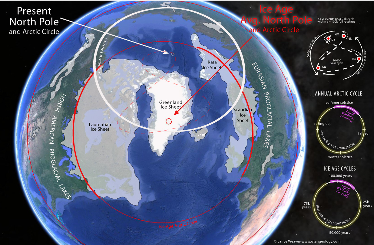
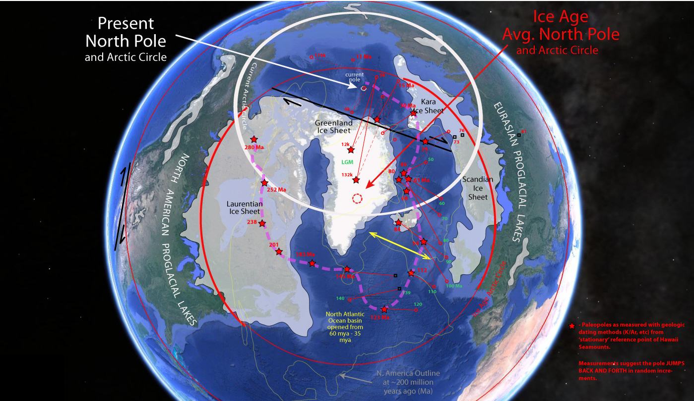
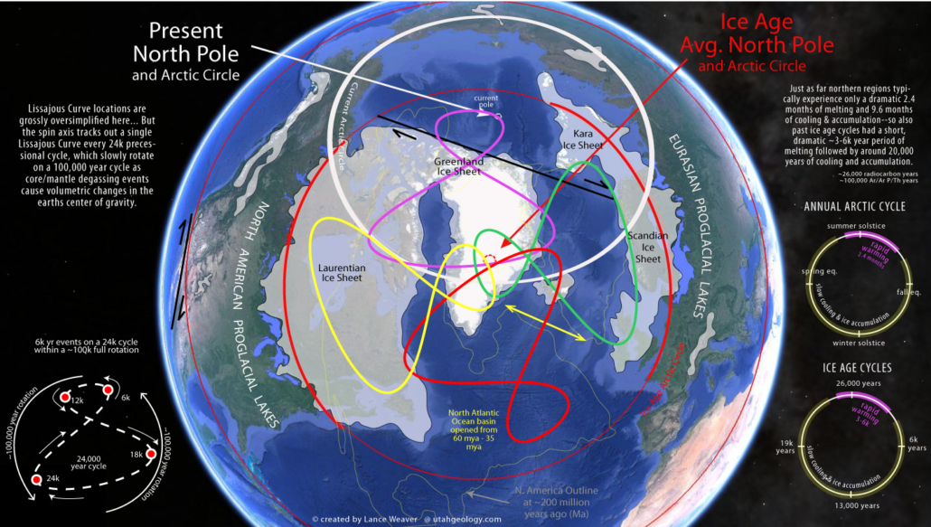
It was during my undergraduate or graduate work toward my degree in geology and geophysics that I first noticed that the majority of Northern Russia, Siberia and Northern Alaska were never fully glaciated during recent Ice Ages. In fact the areas where the last continental ice sheets persisted formed a nearly perfect ‘Arctic circle’ around a pole centered over Greenland.
The more I puzzled over this, the odder it seemed to me that the earth could be cold enough during the ice age for arctic ice to extend to 50 degrees south of the present Arctic Circle and into parts of Illinois and Germany (literally half way to the equator), and yet parts of Alaska and Siberia which are within the present arctic circle were never covered by continental ice sheets or glaciers!
How could this be? For years I’ve searched for a believable answer, always finding the same unconvincing response thrown out. “Siberia & Alaska were an arctic desert, and because of their distance from the sea — storm cells could not carry moisture far enough inland to those areas.” A pretty terrible response in my opinion considering the exact same “arctic desert” conditions would have existed over the 8,000 feet of ice in Central Canada during the Pleistocene, and even currently exist in the center of Antarctica and yet there’s still upwards of 10,000 feet of ice there today! (more on that later) If there’s one thing Antarctica teaches us, its that ice sheets still form in ‘Arctic deserts’ or regions where very little snow falls. It seems in the long run, continental ice sheets have a lot less to do with annual snowfall totals, and a lot more to do with temperatures being low enough to limit melting. More sophisticated answers involving anticyclones, Hadley cells in the jet stream driven by particular ocean currents and intercontinental rain shadows have been offered but are all equally implausible when examined closely. Is there perhaps a more convincing explanation for the geometry of the Pleistocene ice caps?
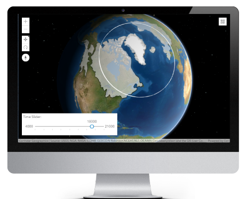
Ice Cover Visualization. Click on the link to see my Ice Age visualization application which shows the extents of the Pleistocene polar ice sheets in a 3D interactive experience. Slide the time slider to see the ice sheet extents though time as well as the theorized track of the north pole. Toggle on & off current & ancient latitude lines as well as an Antarctica overlay. Note the geometry of the ice sheets suggests an ice age north pole centered over Greenland.
TPW Caused by Crustal Precession & Obliquity Forcing as a Replacement for Milankovitch Cycles
Most scientists are well aware that magnetic north migrates its way along the surface of the earth every year. It’s what makes navigators have to change the declination of their compasses every year. But there’s a big difference between magnetic north and true north. Magnetic north affects only compasses and the earth’s magnetic field, but true north or the geographic north pole is the center of the earth’s spin axis and serves as the center point of all earth’s weather patterns. To most scientists, this is an unchanging bulwark of global geography and climatology–changing only over the span of millions of years.
But unbeknownst to the majority of the world, this stalwart feature actually changes each year just like the magnetic pole. It was Swiss physicist Leonhard Euler who predicted in 1765 that the geographic north poles must change based on astronomical observations, but it wasn’t until almost 100 years later when S.C. Chandler published his 1891 papers, laying out more precise calculations for the annual movement of the geographic north pole. His experiments found that the pole moved in spiral circles with a circumference of as much as 200 feet per year. (a radius of 26-33 feet). These ‘Chandler Wobbles‘ as they were dubbed, have been the source of controversy every since, with scientists actively debating their exact cause. Explanations ranging from changes within the earth’s mantel, to atmospheric friction, to changes in ocean currents, groundwater movements and seismic crustal adjustments. In this paper we’ll explore these explanations and offer our own, but more importantly I’d like to propose that this slow true polar wander of the earths geographic north pole, with periodic rapid migrations, is a FAR better explanation for the ice ages, than the current theory. In fact, if Milutin Milankovitch had known that the geographic north pole actually migrates nearly as many miles every decade as the two degrees (140 miles) obliquity nutation he proposed as the leading cause for earth’s 24,000/100,000 year ice ages, perhaps we wouldn’t have to be scratching our heads over why the Pleistocene ice caps don’t match up with our current north pole.
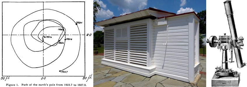
At present the movement of the geographic north pole is mostly in circular motion, with linear movement totaling only about 31.5 inches since it began to be carefully tracked to a GPS level in 1993. But during that period something strange also happened to its linear motion. It went from apparently heading northward during Chandler’s time, to heading westward in the nineties, to recently turning around and heading to Greenland. This is hugely significant because it may be evidence that an unluckily timing of a slowing, stopping and reversal of the geographic pole wandering that is responsible for the ice ages just happened to coincide with modern precise tracking of the pole, causing us to miss the ‘would-be obvious fact‘ that this is the tail end of the driving mechanism for long term global glacial and interglacial periods!
In fact, even without episodic rapid wandering events, when we do the math to figure out how fast the pole would have to move between each glacial & interglacial period to account for the fact that Pleistocene glaciation appears to be centered over southern Greenland, we find that the change of about 1,700 miles over 50,000 years gives an estimate of about 179.5 feet per year. That’s less than the circular movement of the Chandler wobble, so certainly within the realm of possibility!
So to really explore this likely possibility that the geographic north pole has migrated or nutated between the area of southern Greenland and its present location on a cycle of around 24,000 years lets go over an overview of:
- What the ice ages are.
- How they come and go.
- How we know about them.
- What we currently believe causes them. (
- Why geographic polar drift with episodic rapid wander is a FAR better explanation of the data.
- The driving mechanism for changes in precession & obliquity & why the core changes at a different rate from the mantle.
- How it fits into the larger geologic history of True Polar Wander (TPW) and glaciation.
- Its implications on modern global warming and Climate Change models.
What are the Ice Ages
Although it’s well known to most, the Ice Ages refer to periods in Earth’s history when large parts of Europe & North America were covered in continental ice sheets and glaciers. Early scientists assumed these periods were characterized by significant drops in global temperatures which led to the expansion of ice across these continents. The terminal limits to these glaciers left large heaps of earth called terminal moraines which were noticed and mapped out by early geologists Study of these deposits eventually showed that the most recent and prominent ice age, often called the Last Glacial Maximum, occurred approximately 20,000 years ago.
Ice ages are part of Earth’s long-term climate cycles, influenced by various factors such as changes in the Earth’s orbit, axial tilt, and the distribution of continents and oceans. These changes affect the amount of solar energy reaching the Earth’s surface, leading to cycles of glaciation (when ice sheets advance) and interglaciation (when ice sheets retreat). The Milankovitch cycles, which describe the variations in Earth’s orbit and tilt, play a significant role in these processes, causing shifts in climate over tens of thousands of years.
The current period, known as the Quaternary Period, began around 2.6 million years ago and includes several glacial and interglacial cycles. The Holocene Epoch, which started around 11,700 years ago, marks the end of the last ice age and the beginning of the current interglacial period. Human civilization has developed during this relatively warm and stable climate.
While the Earth is currently in an interglacial period, scientific evidence suggests that future ice ages are possible, depending on long-term climate trends. However, human activities, such as the burning of fossil fuels, are significantly altering the Earth’s climate, potentially delaying or altering the natural cycles of ice ages.
During an ice age, large ice sheets cover much of North America, Europe, and Asia. The growth of these ice sheets significantly impacts the global environment. Sea levels drop as more water is trapped in ice, exposing land bridges that allow species to migrate between continents. The Earth’s climate becomes cooler and drier, with vast areas transformed into tundra and steppe ecosystems. These environmental changes also influence the evolution and distribution of plants, animals, and early human populations.
Scrutinizing the Prevailing Views
Central Antarctica really is a frozen desert. The Amundsen-Scott South Pole Station, located in the middle of Antarctica typically records only about 0.5 – 3.1 inches of snow (water equivalent) per year. Most of its snow accumulation there is often blown in from the coastal regions where snow fall can be as high as 15–25 inches a year. (Or it falls as frost-like ice crystals instead of snow) The continent as a whole averages only 6 inches of snow a year, and yet still has managed to accumulate 1 to 3 miles of ice over the last 14 million years (5,000-13,000 feet of ice). Compare that to Fairbanks in the center of Alaska which averages around 45 inches of snow a year but zero glacial accumulation — and you can see how its not impressive snowfall totals that form continental glaciers but consistently cold summer temperatures low enough to facilitate less snow melting than gains.
As anyone whose spent much time in alpine environments knows. Its the night time temperatures that dictate when the snow and ice is about to begin its rapid summer melt. Glacial science is complex, but as a general rule, if you want to grow a glacier, all you need is ANY snow and temperatures which are consistently BELOW freezing in the accumulation zone. Places like Prudhoe Bay or Fairbanks Alaska with summer night time temperatures of 40°F to 50°F are simply not cold enough to grow or maintain glaciers, despite their high snowfall totals. On the other hand places like Casey or Esperanza Base in Antarctica, with summer night time temps of 20°F to 30°F, with smaller snowfall totals are.
So how is it then that places like Illinois, New York, Denmark and North Germany with current summer night time temperatures up to 60-70°F, and latitudes of 46° (roughly 5,500 miles from the North Pole), were able to accumulate upwards of 7000-10,000 feet of glacial ice during the supposedly frigid Ice Age. And yet places like North Siberia or Northernmost Alaska, with current summer night time temps as low as 40°F and latitudes within the Arctic Circle (2,500 miles from the North Pole) were not? The current “frozen desert” explanation holds less water than the frozen air that many blame it on. Really, its borderline ridiculous. Especially when you consider places like central Alaska or the Kamachatka region of Eastern Russia. These regions fall at the tail end of strong North Pacific weather cells which massive amounts of moisture from the Pacific to these Northern Latitudes. (Just like Greenland, the North Sea & Scandinavia are at the tail end of the Caribbean Jet Stream which does the same in that hemisphere). To suggest that these coastal regions did not have access to enough moisture to build ice sheets is as unlikely and faulty as the argument that ice sheets need large amounts of snow to build in the first place!
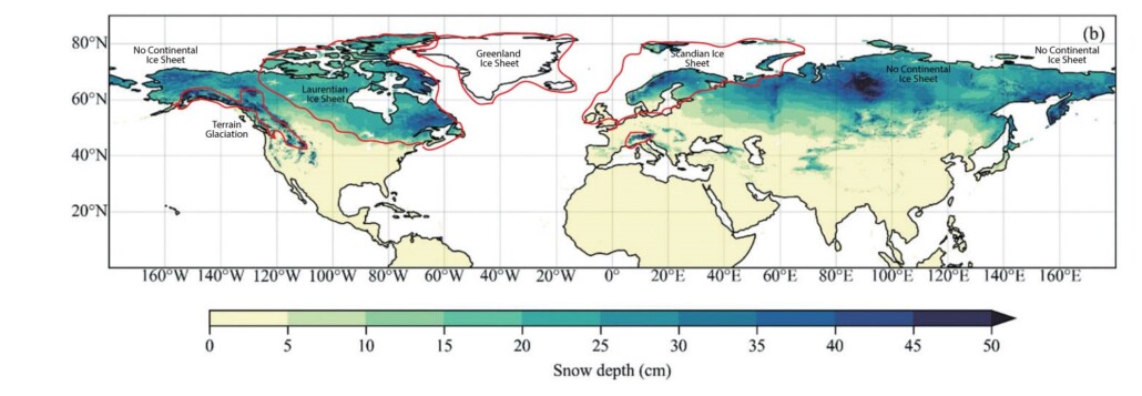
As a great example lambasting both these arguments, look at the annual snow accumulation portrayed from time-lapse satellite imagery of the Northern Hemisphere. The annual snow gains and losses follow latitude almost exactly with the only exceptions being high elevation areas like Greenland & the Rockies. The current winter Arctic desert conditions of Central Siberia make little to no difference in the general trend of annual snow cover. Despite the smaller amounts of snow, high latitude regions like Siberia, Northern Alaska and Arctic Canada are the first to gain snow, and the last to lose it each year (or high elevation regions like Greenland & the Northernmost Rocky Mountains which are cold enough to keep ice all year long).

See the same yearly snow and ice accumulation with sea ice added, and note how it corresponds almost entirely to latitude. Only elevation, as already mentioned, and the Gulf Stream current, which brings warm water from the South Atlantic to the North Sea affects the general latitudinal rule of snow accumulation—making areas of northwest Europe slightly warmer, a trend opposite of what we sea during the ice age.
Glacial geologists sometimes also use processes like the albedo effect, thermohaline oceanic currents and localized microclimates created by ice or large fresh water dumps into constricted oceans to help explain how continental glaciers could have been SO massive and globally lopsided during the Ice Age. As evident in the above snow accumulation maps, every one of these three afore mentioned factors obviously have only little effect on modern day glacial or ice sheet growth. Truly the lack of ice in the North Sea caused by the Gulf Stream is the only real example of a microclimate created by ocean currents which breaks the general latitudinal rule of snowfall and snow/ice persistence. And even its strong effects only change latitudinal snow persistence by around 15 degrees latitude—and even then the effect is restricted primarily to marine ice and coastal environments.
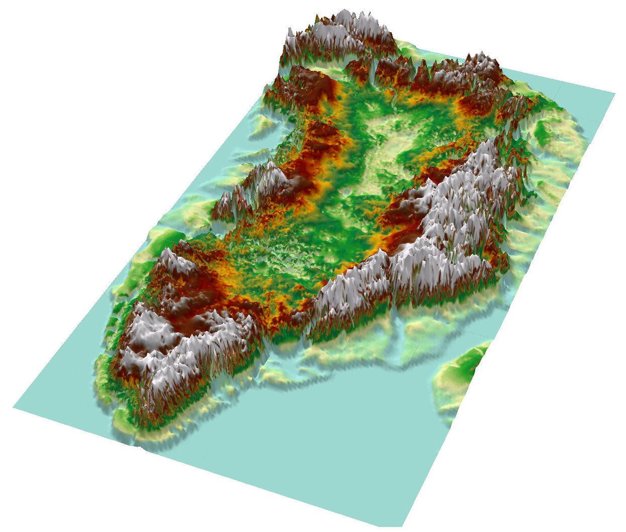
Some have suggested that Greenland’s ice sheet existing at such a southern latitude is another exception to the latitudinal rule of snow persistence, however, I find those who see Greenland as a glacial anomaly, haven’t actually studied the elevation profile of the continent in order to see how the high the mountain ranges which literally surround the continent are (especially the southern tip of the continent which extends out of the arctic circle). These mountains are the obvious explanation for why Greenland has maintained an icecap post-Pleistocene at latitudes farther south than adjacent iso-latitudinal ice sheets. And were the formation of the Greenland ice sheet or its persistence predominately any of the other three reasons (albedo effect, oceanic currents or localized microclimates caused BY the ice) we would SURELY have had a similar Pleistocene ice sheet in the Kamchatka region of Eastern Russia or an existing persistent ice sheet somewhere in Siberia or Eastern Russia since it would have been subject to the same Albedo Effect — and to this day consistently has one of the coldest non-glacial microclimates on earth!
Growth & Melting of Ice Age Ice Sheets
Now let’s compare the above snow accumulation animations to an animation of the glacial ice growth and retreat during the last ice age. Pleistocene snow and ice accumulation and melting followed an entirely different pattern than it currently does. In fact it is striking how obviously the ice sheets seem to point toward a geographic north pole in the region of Greenland.
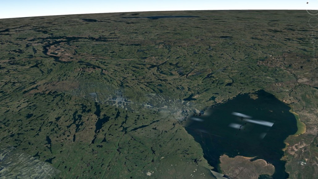
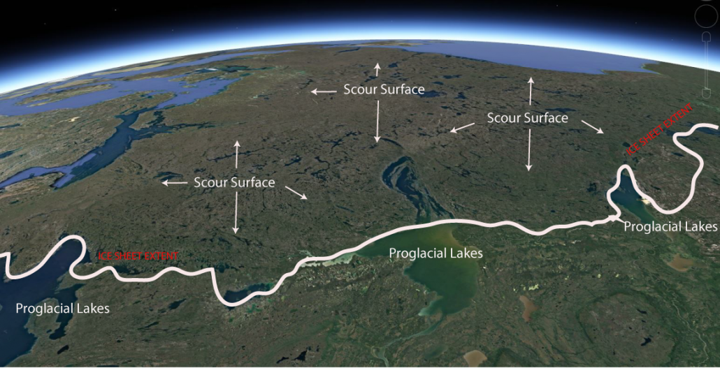
There’s a lot of misunderstanding among the unstudied general public on exactly where the great northern Ice Sheets were and were not during the ice age. (There is near total agreement among trained glacial geologists). This public misunderstanding is mostly the result of poor illustrations based on imagination instead of science. Among experts the northern Ice Sheets and their terminal moraines have been well mapped & dated, with the features proving past continental glacier’s locations being well understood. In fact, in addition to the typical continental glacier telltale signs such as bedrock scour, eskers, outwash plains, drumlins and the like—proglacial lakes, which are lakes formed either by the damming action of a moraine during the retreat of a melting glacier, or in the case of continental icecaps, by meltwater trapped against an ice sheet due to bedrock abrasion and major isostatic depression of the crust around the ice are highly visible indicators showing the maximum extent of the thick margins of northern continental glaciers. Look carefully at the following two satellite images noting that the white line marks the average periphery or terminus of the Each of the hemispheric ice sheets, and the white transparent region symbolizes the continental ices sheets themselves. The labeled lakes are terminal “proglacial lakes” formed along the margin of the ice sheet where not only maximum snow fall typically occurs, but also where maximum melting and scouring occur (because weather systems typically drop their moisture most heavily on the peripheries of ice sheets which warm and cold air masses meet).


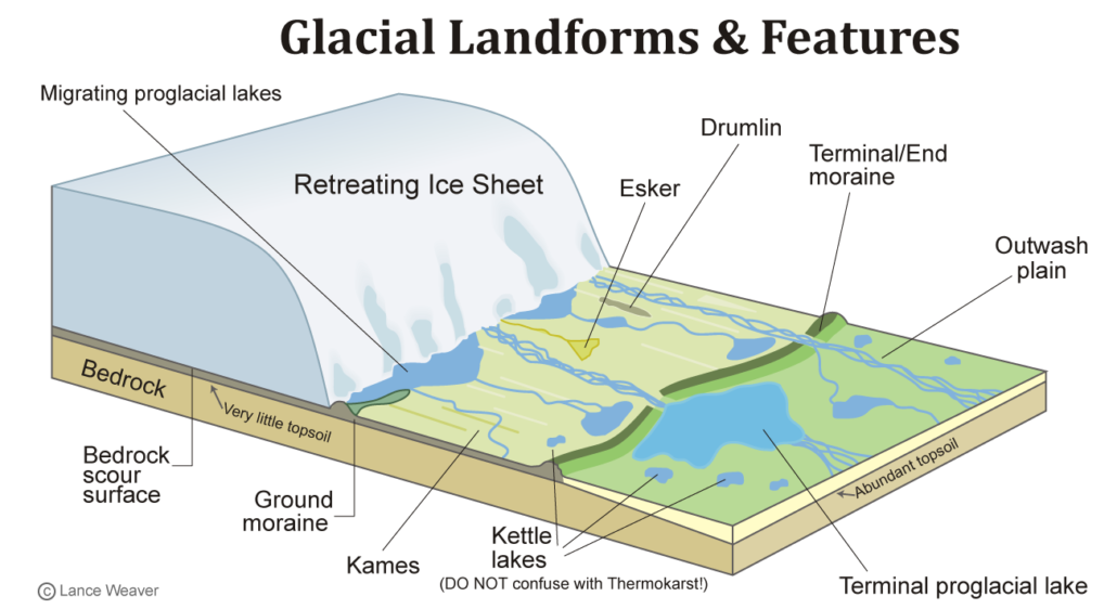
Understanding Glacial Landforms
Before we dive into an explanation of proglacial lakes and the glacial landforms that help geologist know for certain where the polar ice caps were and were not, lets quickly go over the definitions of a few important glacial features.
GLACIER: A glacier is any persistent body of dense terrestrial ice which moves under its own weight. The term was created from the Old French “glace” or “ice” with a Savoy dialect ending likely denoting movement. Sea ice and lake ice are not glaciers. Neither is a thin ice layer under a thick snowpack that hasn’t started to move and plastically deform. Really, by definition a glacier needs ice thick enough to begin to shape the earth beneath it.
ICE SHEET: An ice sheet (which is often used interchangeably with the word ‘Continental Glacier’) is more specifically an area of glacial ice that covers land (not sea) to an extent greater than 50,000 square kilometers (or 20,000 square miles). That’s roughly the size of West Virginia, Costa Rica or Bosnia. This somewhat arbitrary acreage was chosen in order to differentiate Ice Sheets from smaller Ice Caps or alpine glaciers. There are only two Continental “Ice Sheets” on earth—Greenland and Antarctica.
ICE CAP: An ice cap is a bit of a misnomer and thus often wrongly used. It is not the ice which “caps” the the poles of the earth. It is the ice which “caps” a mountain and usually feeds a series of glaciers around its edges. Ice caps are smaller than 50,000 square miles. However, the term “polar ice cap”, referring to the Antarctic Ice Sheet, Greenland Ice Sheet and Arctic Sea Ice is used so frequently in the media that it is generally recognized as an acceptable use… even though it is technically incorrect.
APLINE GLACIER: An alpine glacier or mountain glacier is a glacier which persists because of the effects of lower temperature with higher elevation and exists only within the constraints of a canyon, valley or topographic low. Alpine Glaciers often originate from mountain Ice Caps or even Ice Sheets. The peripheries of the Greenland Ice Sheet & Antarctica Ice Sheets are riddled with Alpine Glaciers exiting from mountainous canyons to the sea. However, its important to note that in the context of my articles, Alpine Glaciers are differentiated from the Continental Ice Sheets because without the mountains from which these glaciers originate, they would have never existed. This in contrast to the Continental Glaciers which form at or near sea level as a result of latitude instead of elevation.
PROGLACIAL LAKE: A proglacial lake is a lake which forms at the downhill termination of a glacier. Proglacial lakes at the terminus of Alpine Glaciers are far smaller than the MASSIVE proglacial lakes formed at the terminus of Continental Ice Sheets. Proglacial lakes form in large depressions caused by glacial scouring. In massive ice sheets proglacial lakes often form as a result of isostatic depression from the weight of the ice.
GLACIAL SCOUR SURFACE: When ice sheets move over relatively level surfaces, inconsistencies in the hardness of the bedrock create a distinct topography of lakes and linear erosional features called striations. In the case of Alpine Glaciers, these features can be small — ranging in size from a few centimeters to tens of meters. With Ice Sheets, however, these lakes and striations are often hundreds of meters or kilometers long and visible from space. Glacially scoured topography is one of the most obvious ways geologists know where a continental Ice Sheet existed. In places like the Canadian Shield or Scandinavian Shield the glaciers left a VERY distinct topography where nearly ALL topsoil and recent geological layers have been scoured away, leaving behind a distinct landscape of lakes, old bedrock and exposed linear features matching the movement of the ice mass.
DRUMLIN: A long, low hill of sediments deposited by a glacier. Drumlins often occur in groups which are referred to as drumlin fields. The narrow end of each drumlin points in the direction of an advancing glacier.
ESKER: A winding ridge of sand deposited by a stream of meltwater flowing underneath the retreating glacier.
KETTLE LAKES: Lakes which form from chunks of ice left behind from the retreating glacier.
GLACIAL PLUCKING: Plucking, also referred to as quarrying, is when a moving glacier exploits pockets of poorly consolidated bedrock or sediment, ‘plucking’ out a depression which later often forms a lake or pond in the substrate. Plucking is a process which helps to create distinctive Glacial Scour surfaces.
THERMOKARST/PERMAFROST LAKE: Often confused with kettle lakes or glacial landforms, Thermokarst lakes ARE NOT glacially formed! Also called a permafrost lake, thaw lake, tundra lake, thaw depression, or tundra pond, it is a body of freshwater, usually shallow, that is formed in a depression formed by thawing ice-rich permafrost in a tundra environment. They are very prevalent in Northern Alaska & Siberia. A key indicator of thermokarst lakes is the occurrence of excess ground ice with soils having an ice content greater than 30% by volume. They commonly form in ancient ‘oxbow lakes’ and deltaic deposits and form as pockets/aquifers of gravel freeze and thaw— both heaving/elevating the surface of area of greater groundwater content (causing surface erosion) and simultaneously collapsing the underlying substrate from the weight of the ice. (Chemical dissolution of underlying soils can also come into play–thus the ‘karst’) When this pocket of ice melts, a thermokarst or tundra/permafrost lake is left in its place. They are differentiated from glacial landforms by their shape, sediment composition and absence of any other accompanying glacial landform.
Once you understand the basics of these glacial features, its easy to simply use Google Earth to explore the regions shown above to make your own conclusions concerning the location of the Pleistocene Ice Sheets. I literally have not shared this with another individual who is even moderately trained in recognizing the preceding glacial landforms who has not come to the same conclusion that the location of Pleistocene Ice Sheets and absence of Glacial landforms in Northern Alaska and Siberia seems hard to explain without evoking some type of True Polar Wandering event. The difficulty and debate comes in when geologist try and decide, how on earth a True Polar Wandering event could have occurred in this short timeframe! These types of events become VERY debatable & problematic for professional scientists when attempting to use any type of catastrophism to explain. Why? I’ll explain in the next section, but first lets look at a satellite images to solidify in our minds the exact location of the Pleistocene ice sheets.
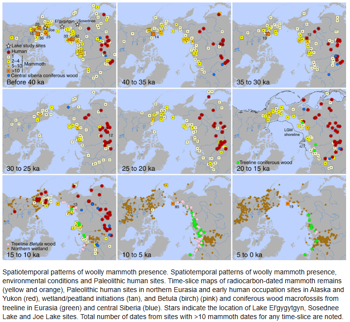
In addition to geologic evidence, archaeological evidence helps us to know clearly where the continental glaciers were and were not. For instance, incorrect ‘neat-looking’ maps like the following one from technistuff, which try to suppose that the thermokarst regions of Siberia were actually glaciated are definitively proven false by the vast amount of archaeological evidence of Megafauna found within those same karstic sinkholes of Siberia and the Yukon Territory of Alaska. Literally thousands of megafauna remains, as well as even human remains show that these areas were not only NOT glaciers during the bulk of the ice age, but were habitat for abundant plants and animals.
Bonkers Pseudoscience? Or is there Something to this?
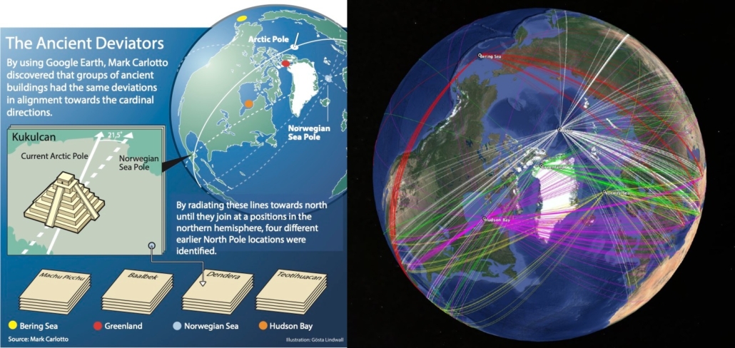
Authors like Mark Carlotto and Mario Buildreps propose the radical “Ancient Pole Hypothesis,” which argues that hundreds of archaeological sites—whose current alignments appear random or non-astronomical—were actually oriented toward previous locations of the North Pole. By utilizing spherical trigonometry to “reset” the global grid, they suggest that sites like Teotihuacán or the Great Ziggurat of Ur were built upon the foundations of OLDER sites which align with former geographic poles in Greenland, Norway, or the Aleutian Islands, implying that the buried foundations of these structures are far older than mainstream archaeology suggests. Their work builds on the debunked ideas of Charles Hapgood, who posited that a series of “crustal displacements” events shifted the Earth’s lithosphere in sudden catastrophe and that the alignments we see today are actually a preserved record of the planet’s previous rotational orientation.
I’ve followed the work of these authors dismissively for many years now, being hung up on the impossibility of the obviously wrong timelines and exact locations of their poles. But I’ve become convinced that there really is something to the idea that many iron and bronze age archaeological sites were actually built upon the foundations of smaller buildings and pyramids (now buried in the cores of these structures), or in some cases on the massive ancient foundation stones of sites which date to the period between the end of the Last Glacial Maximum (15,000 years ago) and ~3,000 years ago when the pole finally migrated/jumped it to its current location.
Likewise author Mario Buildreps….
.
UNDER CONSTRUCTION FROM THIS POINT ON.
True Polar Wander as a Mechanism for Rapid Deglaciation
Both gradual and relatively rapid true polar wandering events are well established in paleomagnetic data throughout the geologic record. However, established methods used for dating the paleomagnetic evidence for these events has generally yielded time frames much greater than my hypothesized ~20 degrees of movement in >3000 years.
True polar wander is an known effect of non-symmetrical objects with multiple moments of inertia also known as intermediate axes. Because of the equatorial bulge and large mantle plumes, the mass distribution of the Earth is not spherically symmetric, and the Earth has three different moments of inertia axes. The axis around which the moment of inertia is greatest is closely aligned with the current rotation axis (the axis going through the geographic North and South Poles). A second axis is near the equator through the equatorial bulge. A third is theorized to also cross the equator at a right angle to the second, although mantle plumes and crustal imbalances from mountains or ice could cause it to locate elsewhere. However, if the moment of inertia around one of the two axes close to the equator becomes nearly equal to that around the polar/rotational axis, the constraint on the orientation of the object (the Earth) is relaxed. Even slight imbalances can make the Earth (both the crust and the mantle) slowly reorient until one of the second moments of inertia moves to the rotational axis or North Pole, with the axis of low moment of inertia being kept very near the equator.
Details on true polar wander in relation to paleomagnetic data is explained in this video lecture by Dr. Trond Torsvik (CEED, University of Oslo, Norway) who has worked on paleomagnetics for nearly three decades. (TPW explanations start at minute 38:16)
A MUCH FASTER example of this effect is explained in detail in the following Veritasium video on The Bizarre Behavior of Rotating Bodies. The same concept of multiple moments of inertial also slowly rotates planets over time.
Dzhanibekov Effect (pronounced genibekov) is often used by catastrophists as an example of how rapid polar wondering events might occur over small timeframes. It’s important to realize however, for such theories to be viable, the rotation between the two moments of inertia or bipole stability points MUST BE SLOW ENOUGH to keep inertial forces below thresholds that could rip the earth in pieces or kill everything on its surface. With an equatorial speed of about 1,000 miles per hour, rotational momentum could not exceed about 5-10 miles per hour without causing earth-changes contradicted by geological extinction data, orogenic event data, climate data, and more. At 5-10 miles per hour, it would take 4-8 days for a pole to shift 1000 miles, and 25-50 days to travel 6000 miles from the pole to the equator. Most geologists would suspect if the Dzhanibekov Effect plays a role in rapid True Polar Wander, we’d be looking at much slower changes over centuries to millennia. (Especially given that our most recent extinction events in the Pleistocene seem to have affected the poles far more than the equator, killing off high latitude megafauna and leaving african equatorial megafauna. The EXACT OPPOSITE effect we’d expect if polar momentum shifted rapidly enough to cause large tsunamis–which would be worst at the poles) see: https://www.youtube.com/watch?v=Xrf1HzFJ8jc
Another possible minor driving mechanism for True Polar Wander could be slight electromagnetic Lorentz forces from the heliosphere onto earth’s core.
Note that the above physics principles are remarkably similar to the Larmor Precession of atomic nuclides and I believe has something to do with the true relationship between true polar wander and the precession of the equinoxes as I explain a bit later in the document as well in my article ‘Is the Orbit of Jupiter related to Solar Cycles‘ .
Large low-shear-velocity provinces (LLSVP’s)
Large low-shear-velocity provinces (LLSVPs), also called large low-velocity provinces (LLVPs) or superplumes, are characteristic structures of parts of the lowermost mantle, the region surrounding the outer core deep inside the Earth. These provinces are characterized by slow shear wave velocities and were discovered by seismic tomography of deep Earth. There are two main provinces: the African LLSVP and the Pacific LLSVP, both extending laterally for thousands of kilometers and possibly up to 1,000 kilometres vertically from the core–mantle boundary. The Pacific LLSVP is 3,000 kilometers (1,900 miles) across and underlies four hotspots on Earth’s crust that suggest multiple mantle plumes underneath. These zones represent around 8% of the volume of the mantle, or 6% of the entire Earth. The LLSVPs lie around the equator, but mostly on the Southern Hemisphere. Global tomography models inherently result in smooth features; local waveform modeling of body waves, however, has shown that the LLSVPs have sharp boundaries.
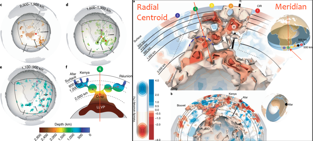
Sometimes related to the LLSVP’s are mantle plumes. A mantle plume is a giant, column of extremely hot, buoyant rock rising from deep within the Earth’s mantle, often near the core-mantle boundary, that punches through the lithosphere to create volcanic hotspots and large volcanic provinces, like the Hawaiian Islands or Yellowstone. These plumes stay relatively fixed, while the tectonic plate above them moves, leading to chains of volcanoes forming over time as the plate slides over the plume. Combined, these two large mantle structures create irregularities in the otherwise uniform mass of the earth and could act as bipoles, or multiple moments of inertia able to threaten the stability of the rotational axis.
Understanding Long Term Trends of True Polar Wander (TPW)
Nothing about True polar wandering, is controversial or unaccepted by geologists, geomorphologist and paleomagnetism researches in the mainstream scientific community. What IS controversial is rapid true polar wandering events spanning timeframes of less than a million years or so. Certainly my timeline of a few hundred to a few thousand years for a true polar wandering event will evoke debate. Toward the end of his life Albert Einstein appears to have been thoroughly convinced by many of Charles Hapgood’s arguments regarding rapid pole shift and perhaps even catastrophe. Einstein wrote in the foreword to Hapgood’s book, Earth’s Shifting Crust, “in a polar region there is continual deposition of ice, which is not symmetrically distributed about the pole. The earth’s rotation acts on these unsymmetrically deposited masses and produces centrifugal momentum that is transmitted to the rigid crust of the earth.” For Einstein and Hapgood, the very off-center weight of the northern ice sheet itself seemed a plausible mechanism to cause a rapid pole shift. Geologist (including myself), however, are not convinced. Not only did Hapgood’s brand of catastrophism seem too much like creationism, It simply did not explain the configuration of mid-oceanic spreading ridges, marginal continental subduction zones with their associated volcanic arcs and constant earthquakes, as well as evidence for the slow uplift of so many of earth mountain chains as well as Wagner’s Plate Tectonic Theory did. Nor does it consider the science of True Polar Wandering. Thus Hapgood’s theories were dismissed and discarded to await a future date when a new group of scientist more removed from the nineteenth and twentieth century passionate debates between uniformitarians and creationists, could relook at the evidences of Hapgood & Einstein and see if perhaps there was a combination of uniformitarianism and true polar wander that could explain the many arguments given in Hapgood’s work.
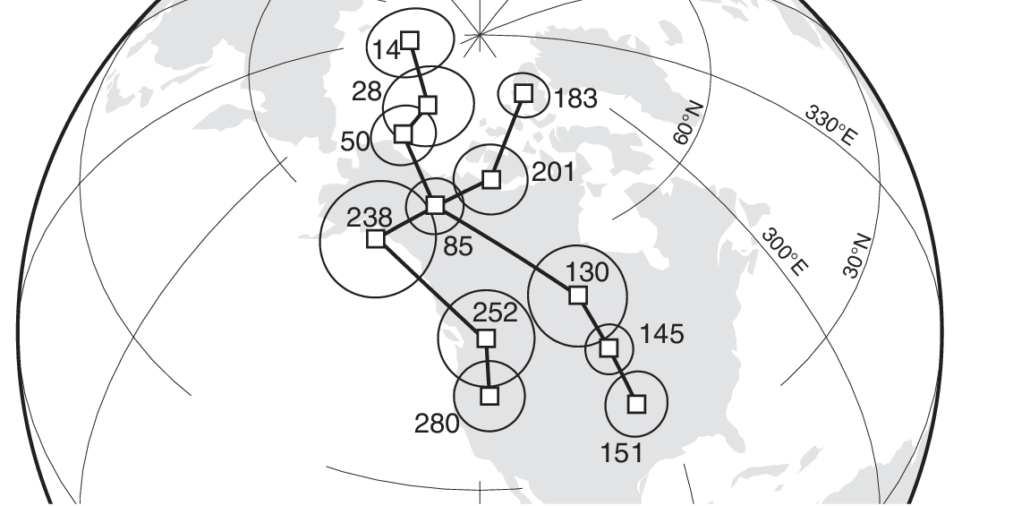
To Do. The most important part of the above Sager & Kopper illustration is the back and forth (east/west) skipping of the pole perpendicular to the long term motion of pole travel (north). I need to add that to my main illustration, and note that long term motion is no longer north, so back and forth skipping is likely now north/south between north greenland and current location!
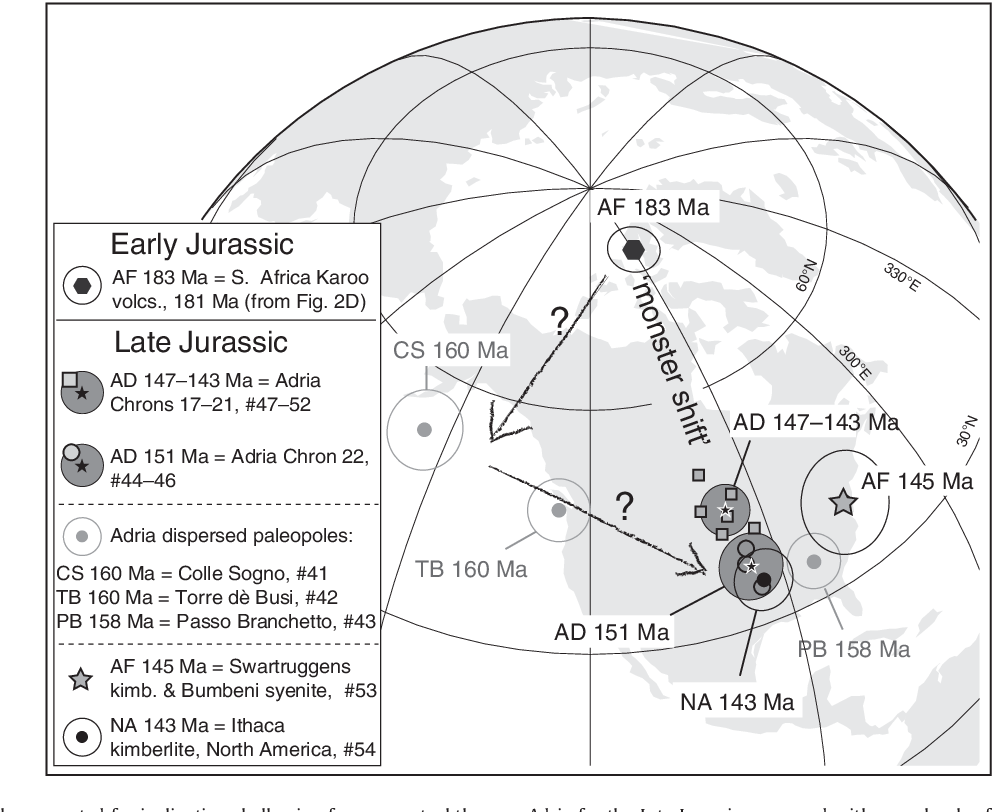
(Above. from The drift history of Adria and Africa from 280 Ma to Present, Jurassic true polar wander, and zonal climate control on Tethyan sedimentary facies Muttoni, et al, 2013)
My illustration showing pole locations and TPW (purple dashed line) since the cretaceous. Perhaps one of the most important aspects of this illustration, adapted onto a globe from the William Sager & Kopper article above, is the back and forth (east/west) skipping of the pole perpendicular to the long term motion of pole travel (north) found by comparing pole locations in the Hawaii- Emperor sea mount chain. Within that motion are numerous ‘anomalous’ pole outliers which suggest rapid wander.
In my model I’ propose the above long term average pole location is actually superimposed onto a short-term motion that traces out large circular or Lissajous Curve motions created by gravitational forces of the earth’s precessional cycle. In the next section I will lay out my theory of precession actually causes rapid true polar wander, when combined with periodic intersection with galactic wave fronts (seen as columns of non thermal galactic filaments).

View in Full Screen Open in new window
Very rough representation of polar motion. Due to constraints in the program code, the motion is not completely accurate, but close enough. The largest order circle should be FAR smaller, the movements are FAR less regular and more erratic and jumpy because of changing random variables, the lissjous curve should be more oblong like shown in the background and above images and it changes each cycle anyway.
.
Lissajous Curves & TPW Paths
Actual spin axis or north pole location paths almost certainly follow a path traced out by one of the lower order Lissajous Curves. Lissajous curves are complex, looping patterns traced by a point mapped out between the intersection of two separate rotating/circular controls, named after Jules-Antoine Lissajous, French physicist who studied them in the 1850s. These mesmerizing shapes, also called Bowditch curves, form familiar figures like lines, circles, ellipses, or intricate loops, depending on the frequency ratio (e.g., 1:2, 3:4) of the two oscillations, with rational ratios creating closed curves. They visualize sound, compare electrical signals on oscilloscopes, and appear in physics, art, and music.
They are formed by projecting the sum of two circular motions onto a flat plane, and as such are the type of shape or motion expected from rotational irregularities in the earth’s orbit projected onto the polar spin axis plane. Differences in the shapes arise from the unique combinations of DIFFERENCES IN SPEED OR VELOCITY of the two governing circles used to project the composite Lissajous shape. (see YouTube video illustrating how they are created). For example, if the northern pole begins wobbling FASTER than the southern pole, a shape such as those we see in row #1 below is formed (east west squiggles). If the opposite condition of a southern hemisphere pole wobble being faster than the north occurs, shapes like those mapped out in column #1 are formed (north-south squiggles). If both poles rotate at equal velocities, a perfect circle such as that seen in the diagonal from upper left to lower right is seen.

.
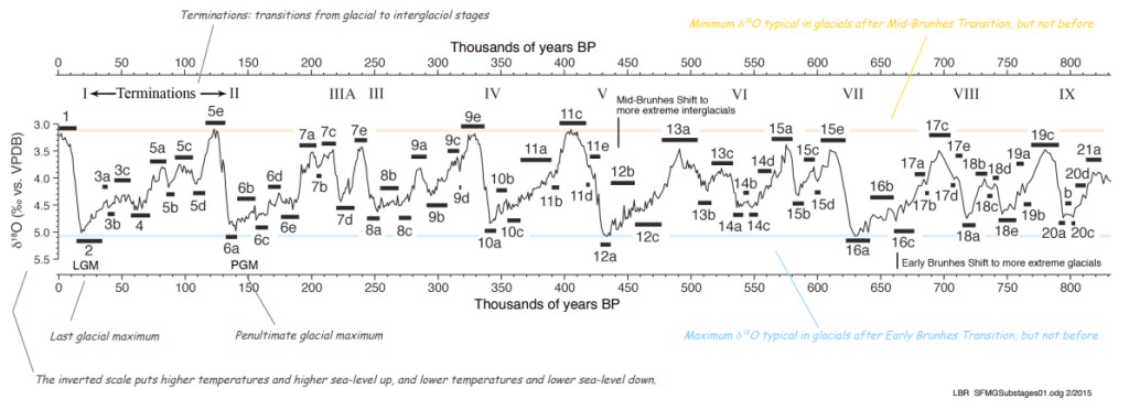
Polar See-Saw, D-O Events & Ice Core Data for TPW
Seesaw Heinrich Stadials as 3k Year Wobble Events
The ‘Bipolar Seesaw Hypothesis‘, or Anti-Phased Climate Events Between Greenland and Antarctica IS STRONG evidence for a wobbling pole. Heinrich event and Dansgaard–Oeschger event / Bond Event data supporting this hypothesis shows Antarctica warming while Greenland cools. It’s also strong evidence that the current dating methods are somewhat correct for the last 120k, and that Antarctic cores really are much older than Greenland cores. In my hypothesis, I would argue that each HS/GS/AIM event represents a 3000yr oscillation. (with smaller & larger oscillations of ~3000yr,~1470yr, ~735yr)
We should probably allow for the possibility that every HS/GS event represents 6000 or 700 or 1400 year events if the radiocarbon dates are wrong. Especially since we don’t really see these events for the last 12,000 years since the end of the ice age, which they interpret as being being because they don’t happen during interglacials. But maybe its a dating problem? (probably not)
Dansgaard–Oeschger (D-O) events: (occur every ~3k yrs) are rapid climate fluctuations, recorded in the Greenland ice cores, where changes in oxygen isotopes (δ18O) indicate sudden warming (the start of the event) followed by a gradual cooling. 14.7k, 23.3, 27.8, 30.8, 32.5, 35.3, 38.3, 40.0, 43.1, 46.1, 47.7 etc..
Antarctic Isotopic Maxima events (AIM): Opposite abrupt, significant temperature 3k yr warming events in Antarctica which form the southern dataset for the polar sea-saw DO events. AIM 4 & 24 were HUGE, at 29k bp and 105/128k bp.
Heinrich Stadials (HS-events): (occur every ~9.2k) are massive discharges of icebergs from the Laurentide Ice Sheet into the North Atlantic, causing widespread cooling. 12k, 16.8, 24.1, 31.7, 38.2, 47.9, 59.5, 67.2, 79.5, 95.0
Greenland Stadials (GS): (occur every 3.14k) are the cold periods recorded in the Greenland ice cores, which often correspond to the time between the D-O warming events. 12.8k, 23.9, 28.2, 31.5, 33.1, 36.3, 38.6, 40.8, 43.6, 46.9,
Bond Events: (occur every 1470yr/2940yr) are North Atlantic geological ice rafting events studied by Gerard C. Bond based on petrologic tracers of drift ice in the North Atlantic.
Marine Isotope Stages (MIS): Alternating warm and cool periods in the Earth’s paleoclimate, deduced from oxygen isotope data derived from deep sea core samples. Even numbers have high levels of oxygen-18 and represent cold glacial periods, while the odd-numbered stages are lows in the oxygen-18 figures.
This evidence of a 3000 year reoccurrence of climate oscillations seems pretty significant, as it matches perfectly with Oahspe and Law of One dates for the last ‘Major Cycle’ where man is on earth. Also if the NGRIP Greenland 140k is actually 75k, then Antartica’s 800k seven cycles is probably 7 x 75k which would be 525k which would likely correspond with the Oligocene, when geologic evidence shows glaciation started. So if the Oligocene was actually 500k years ago, the Cambrian would probably be in the 2-4mya range, WHICH IS A FAR BETTER DATE FOR THE AGE OF THE EARTH. I should be able to use magnetic reversal chron ages to do a better correlation (assuming that the poles reverse every 3k, 12k or 24k. Geochron studies show the last reversal 40k years ago and 183 reversals from 0-84mya (the last superchron in the Cretaceous) — So I’d assume they happen every 12k which would put 84mya at actually 2 mya. CRETACEOUS AND KIAMAN (permo-conboniferous) SUPERCHRONS WERE PROBABLY FROM GOING THROUGH SUPER ENERGETIC ARMS OF MILKY WAY GALAXY. (Oahspe just calls them ‘Semu Nebula’ where carbon organics fell to earth–which also could shield us from electromagnetic realignments?)
This model could REVOLUTIONIZE geologic dating, using galactic waves which cause geochron reversals as absolute dates instead of radiometric dates which we suggest change massively during these 3k/12k energy events.
NOTE THIS IS HUGELY IMPORTANT… WATCH the youtube video up above on proton precession again. NOTICE the south pole stays pretty stationary, and the north pole precesses. THIS IS WHY ANTARTICA DIDN’T MELT but Greenland DID. So the cumulative Solar & Galactic field (combined with our earth’s magnetic characteristics) dictate our precession, and like THE LAW OF ONE states, for the last 75k, we’ve had 3rd density characteristics dictating a similiar system.
So likely:
-Every 3k we have a geomagnetic excursion, a solar burp, and a small expansion episode
-Every 6k we likely have a bigger excursion, bigger burp, bigger expansion, enough to…
-Every 9k or 12k are the biggest that end ice ages, and we hit the half way point of a full circle.
-Geomagnetic excursions should also occur each 3k, but FULL REVERSALS are sporadic and unpredictable. (except that if they happen, then they happen ON the 3k events)

.
Eyeball counting of varves in cores has ONLY been done down to 40-60k BP. EVERYTHING EARLIER is being inferred by wiggle matching methods.

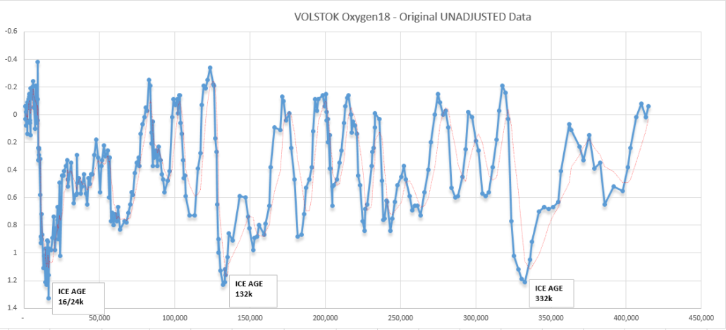
My Excel Graph made from raw unadjusted Greenland Oxygen Isotope data (online Sheets version here).Most notable feature is that there IS NO notable 20k cycle here. Instead its more like a 3-4,000 yr cycle. (see excel sheet for averages)
ALSO NOTE THAT THE 100K WARM PERIOD DOES NOT HAVE TIMES FOR SOME REASON. Its in the data at the end of the dataset that has borehole depth but no assigned time. Why might that be? I added pretend dates of every 250yrs. But note that both the bookends of this data are a bit suspect. If we take them at face value, the most notable feature is the 2/3k periodicity. BUT IT IS NOT STRONG ENOUGH periodicity to hang your hat on, and say you trust the timeline just because it has the pretty 3k number in there. AI says there are THREE Greenland deep cores that go past 120k (and three that stop at 110k), so it does seem validated. BUT still there’s a lot of assumptions in ice cores. These might not be annual varves at all. And the sample rate is kind of arbitrary. We need cores that can be continually scanned.
BUT NOTE THAT THE 123K event is a see-saw, it goes from together to opposite in Greenland/Antarctica.
.
.
Unearthing a Viable Mechanism for Rapid True Polar Wander
The polar see-saw (also: bipolar seesaw) is the phenomenon that temperature changes in the northern and southern hemispheres may be out of phase. The hypothesis states that large changes, for example when the glaciers are intensely growing or depleting, in the formation of ocean bottom water in both poles take a long time to exert their effect in the other hemisphere. Estimates of the period of delay vary; one typical estimate is 1,500 years. This is usually studied in the context of ice cores taken from Antarctica and Greenland.
.
Geologic Marine Isotope Data (MIS)
-Ice ages are nothing like we’ve supposed. They are not coming and going to any large degree. They began to form at the Eocene/Oligocene transition in BOTH the arctic and Antarctic when the Arctic circle was over Greenland (and possibly a few times before since the Cretaceous) and have persisted ever since with short ‘interglacial’. They were caused and ended by the location of the pole, which slowly wanders as a result of TPW driven by inertial forces caused by changes in polar precession. They began with the opening of the Atlantic when Greenland and Scandinavia separated in ~30 mya.
The below illustration shows the major cold periods clearly. It might be helpful to modify the left line to a stepwise angular plot to really show the pole re-organizations. Note the Oligocene and second half of the Miocene are equally cold. (likely signaling ice ages). Eocene and early Miocene are hot houses (likely similar to present). The Pliocene is the one real anomaly where the pole is obviously circulating right over Greenland/Canadian Shield/Scandian Ice Sheet.
On the left line, the Oligocene jog to the left is the Bishop Conglomerate Glacial advance. (Probably the first major glacial period in the west?). The mid-miocene would be the Bull Lake, which then gets warmer and Pinedale would be the Pliocene cold period. The Plio-Pleistocene actually are only about 330k long instead of 5 million years long.
Note O18 ratios are changed purely by latitude! So each shift would shift the ratios.
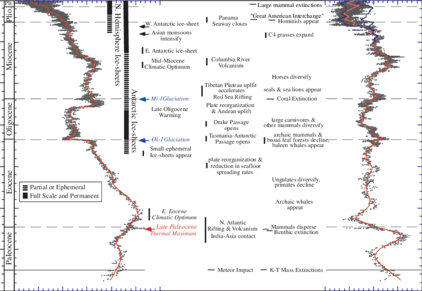
Slightly modified version of the above.

Note: Top line hills are warm periods (such as Paleocene Isotope Maximum and Monterey Event) and down-drops (to the right) are cool off periods (such as Eocene C20, Ol-1 glaciation and Miocene Ser in C5) . I interpret gradual decline as moving pole northward. (O18 ratios are changed purely by latitude!) Main ice ages are 47Ma, 35Ma, 17Ma, 8Ma and 3Ma.
The Below dataset is simply an enlarged subset of the above data. Paper suggests the increased variability since 3mya, could just be higher resolution data.
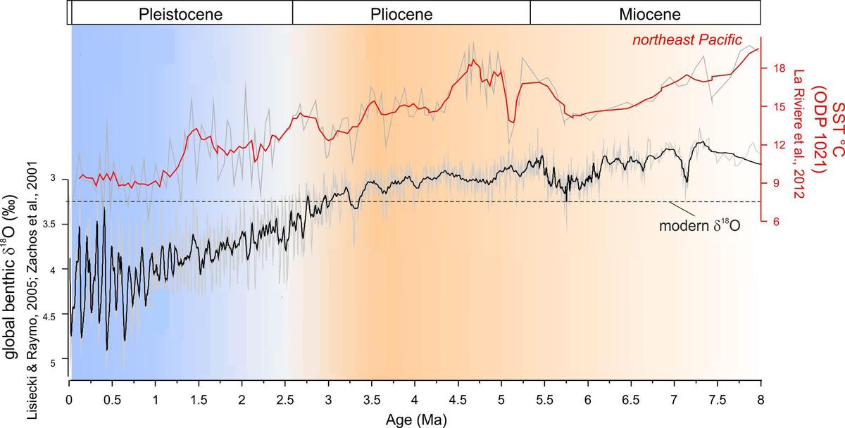
-Oscillations for modern time periods also show JUST AS LARGE of delta/changes in oxygen isotope values. Easily showing 2% to 3% changes in isotope variances. See Knudsen et al, 2011. Figure 4
-Oxygen Isotope values CHANGE WITH SEASON & LATITUDE. That means that as the plates move and the pole drifts northward, the oxygen isotope values change slightly as well. Particularly as you approach the Arctic circle (as you can see from this article, Nakamura, et al, 2014) Note that studies like Hutchinson, et al, 2021, show that Oxygen isotope values can vary from 1 to 2.5% depending on latitude. So when episodes of rapid True Polar Wander occur, it shows as an abrupt change in the oxygen isotope values (such as the Eocene/Oligocene Transition) [find an even better illustration with 6 or 7 locations at different latitudes]
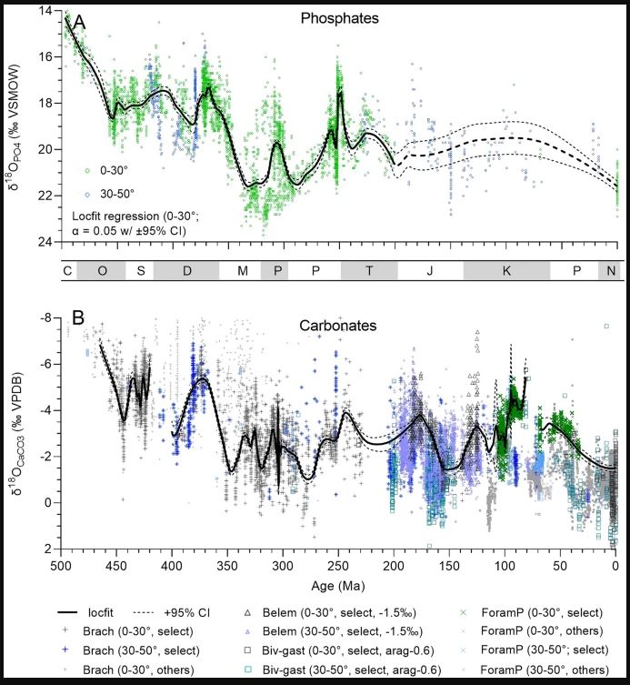
-So How ON EARTH did we get convinced that 3-4% benthic oxygen18 isotope ratios means a glacial/interglacial? Look at figure-1 in this article (shown above). Glaciation in Antarctica started at 2%. If you look at the hot house/ ice house transition in the greater geologic record you can see that the benthic oxygen18 isotope ratios for glaciation/deglaciation in the Carboniferous/Permian to the Cretaceous varies from -2% to -5%, not 3 to 4%.
As listed above… MAJOR COLD PERIODS APPEAR TO BE: Main ice ages are 47Ma, 35Ma, 17Ma, 8Ma and 3Ma.
-Penn/Perm: 270-290Ma
-Mid Cret: 125-133Ma / 140-160Ma
-Late Cret: 83-66Ma. (Maastrichtian, Peak cold @ 80mya)
-Eocene?: 47 Ma (mild) (see this)
-Oligocene: 34-33Ma (Bishop Cg 34-27 Ma, Also Brianhead Fm)
-Miocene: 23-14Ma (17-12Ma)
-Miocene: 7-5.3Ma (7-4Ma, Salt Lake Fm)
-Pleistocene. (glacially dated 0-2.5mya)
In the Uinta’s and much of the Rocky & Sierra Mountains, we see only FOUR major glacial periods. Pinedale, Bull Lake, Pre-Bull lake and Bishop cong. But there is a LOOOOT of erosion between the Bull Lake and Bishop cong. Like 3,000 ft in many places, and the full collapse of Browns Park. These three periods might match with the cold periods seen above in the geologic record. With Pinedale as recent Pleistocene, but Bull lake is actually a Miocene (or both Miocene) glaciation, and then bishop cong is the Oligocene one. Of course this reasoning would require huge problems with late Cenozoic dating (ie. excess argon and radiometric issues) in the west for dating of Yellowstone, Bishop, Valles Calderas (which I’ve already suspected)
A huge issue that this solves is the glaciation of the Eastern Sierras. North of Bishop glaciation is unbelievably obvious and pervasive right to the valley. South of Bishop however, glaciation seems to be destroyed at lower elevations by the Eastern Sierra escarpment fault. (from Bishop to Owens Lake). That SHOULD NOT BE if the majority of the glaciation is POST Miocene/Pliocene faulting. But its exactly what we’d expect if much of the glaciation happened BEFORE late basin and range expansion dropped the East Sierra escarpment fault (which dates from 5-3.5 mya.) The more I look at that area, the more I believe much of that glaciation happened BEFORE THAT FAULTS MAJOR OFFSET 5-3.5mya. Its the same with the Uintas and Utah Laccolith stuff. They lack glacial features, because much of the glaciation happened BEFORE 20-10mya when much of that emplaced.
.
| n.aMERICAN STAgeS | SIERRA NEVADA | ROCKY MTN STAGES | ADJ DATES |
|---|---|---|---|
| End of Late Wisconsin (11-10,000 bp) | Tioga Glaciation Ends (14,000 bp) | Pinedale (13-11,700 bp) | 0-2.5mya |
| Wisconsin Maximum Extent (25-21,000 bp) | Tioga Glaciation Max (21-18,000 bp) | Pinedale Max (22-20,000 bp) | |
| Tioga Glaciation Begins (28,000 bp) | Pinedale Begins (32-30,000 bp) | 0-2.5mya | |
| Beginning of Wisconsin (100-75,000 bp) | Tahoe Glaciation Ends (70,000 bp) | ‘Late Tahoe’ = 50-42k bp | |
| End of Illinoian (130,000) | Bull Lake Ends (130,000 bp) | 7-5.3Ma? | |
| Illinoian Peak (140,000) | Early Tahoe Retreat (145-140k bp) | Bull Lake Peaks (140,000 bp) | |
| Beginning of Illinoian (191,000 bp) | Tahoe Glaciation Starts (170,000 bp) | Bull Lake Starts (190,000 bp) | 7-5.3Ma? |
| Culmination of Pre-Illinoian, i.e., old Nebraskan (300,000 bp) | Sherwin Glaciation Ends | Pre-Bull Lake/Buffalo | 23-14Ma? |
| Beginning of Pre-Illinoian (2.6mya) | Sherwin Glaciation Starts (820,000 bp) | 23-14Ma? |
| Glacial / Interglacial Stage | Approx. Dates (Years Ago) | Marine Isotope Stage (MIS) | Notes |
| Holocene (Current Interglacial) | 11,700 – Present | MIS 1 | The warm period we live in today. |
| Wisconsin Glaciation | 75,000 – 11,000 | MIS 2 – 4 | The last major glacial; reached its maximum (LGM) ~20k years ago. Pinedale Glaciation in West. |
| Sangamonian (Interglacial) | 130,000 – 75,000 | MIS 5 | A warm period, with MIS 5e being potentially warmer than today. |
| Illinoian Glaciation | 190,000 – 130,000 | MIS 6 | A massive glaciation; in the West, this is often called the Bull Lake. ‘Early Tahoe’ in Sierra’s |
| Yarmouthian (Interglacial) | ~300,000 – 190,000 | MIS 7 – 11? | Now grouped into the complex Pre-Illinoian sequence. |
| Pre-Illinoian Stages | 2.6 Ma – 300,000 | MIS 12 – 100+ | Replaces the old “Kansan” and “Nebraskan” labels. |
A great place to test this hypothesis is the Mono Lake area. Are the Bull Lake or Tahoe glaciations positively on top of latest Miocene sediments? There would have been dozens of glacial cycles and advances during the last glacial max… is the geology a mess as far as calling earlier Pinedale/Tioga glaciations Bull Lake/Tahoe? I need to find places where volcanics are interfingering with glacial stages. Is iceland the best place to do this?
.
As you can see, the North American Stages DO NOT match very well with the European stages. Evidence that the pole was skipping around laterally east and west as well as vertically north and south.
| Alps Glacial stages | Great Britain/Ireland | Northern Europe stages |
|---|---|---|
| Würm Glacial End (11,700 BP) | Devensian End (11,700 BP) | Weichselian End (11,700 BP) |
| Würm Glacial Start (115,000 BP) | Devensian Start (115,000 BP) | Weichselian Start (115,000 BP) |
| Riss Glacial End (128,000 BP) | Wolstonian End (130,000 BP) | Saale End (130,000 BP) |
| Riss Glacial Start (300,000 BP) | Wolstonian Start (352,000 BP) | Saale Start (300,000 BP) |
| Mindel Glacial End (347,000 BP) | Anglian End (424,000 BP) | Elster End (370,000 BP) |
| Mindel Glacial Start (476,000 BP) | Anglian Start (478,000 BP) | Elster Start (475,000 BP) |
| Günz Glacial End (621,000 BP) | Beestonian End (478,000 BP) | Bavelian End (866,000 BP) |
| Günz Glacial Start (866,000 BP) | Beestonian Start (780,000 BP) | Bavelian Start (1,000,000 BP) |
.
THE KEY TO CORRELATING ICE AGE DATA TO GEOLOGIC DATA.
Marine Isotope stages are the key to correlating ICE AGE data to Geologic Data. Ice cores are fairly unreliable because of how inconsistent snow fall is. But pelagic oozes are more consistent, and serve as the backbone of ice core data. And Marine Isotope core data goes back all the way through the Mesozoic. And as expected, the stages become less and less per million years as you go back in time. Geologist interpret this as a more hot and stable climate. I INTERPRET IT AS A PROBLEM WITH DATING. In other words, since isotopic decay rates accelerate HUGELY every 3k event, our half life is essentially wrong, so the farther back in time you go, the farther off a lab determined date result is from the reality. I propose that isotopic stages are a better estimate of real dates than radiometic dating results. And if we do the math on isotopic stages we get numbers that better accord with the erosion rates I see on the Colorado Plateau. (ie. 3-5,000 feet of general denudation since the Colorado River found an outlet ~55 million years ago.
To do the math of our new dating method we need to realize that frequency (stages or cycles per Ma) decrease going back in time. Recent stages (last ~1 Ma) are dominated by 100 kyr eccentricity cycles, yielding fewer (~10/Ma). Earlier in the Pleistocene/Pliocene (1–5 Ma), 41 kyr obliquity dominates, increasing to ~24 per million years. Miocene (5–23 Ma) shows similar but coarser resolution (~10–15 per million years). Eocene-Oligocene (23–65 Ma) has even fewer (~1–5/Ma major events), with long-term trends. Mesozoic (pre-65 Ma to 150 Ma) features broad, multi-Ma variations (~0.5–1/Ma), limited by sediment preservation and lower orbital sensitivity in greenhouse climates.
The following chart helps us estimate actual dates from isotopic stages by averaging the number of stages per million years and going back in time.
| Time Interval | Approx. Stages/Cycles per Ma | Key Notes / believed length per cycle | Length if each stage is 3k yrs. |
|---|---|---|---|
| 0–1 Ma (Late Pleistocene) | ~28 stages | 100 kyr eccentricity; high-resolution from ice cores/sediments. | 84,000 years (my theory) OR 616k yrs? (@22k) |
| 1–2 Ma (Early Pleistocene) | ~34 | Transition to 100 kyr; still some 41 kyr obliquity influence. | 102,000 years OR 748k yrs? (@22k) |
| 2–3 Ma (Pliocene-Pleistocene) | ~25–30 | 41 kyr obliquity dominant; more frequent shorter cycles. | 81,000 years OR 594k yrs? (@22k) |
| 3–5 Ma (Mid-Pliocene) | ~20–25 | 41 kyr cycles; warming trend reduces amplitude. | 66,000 years OR 506k yrs? (@22k) |
| Plio-Pleistocene Total: | 112 stages | total of above states & years. | 333k years OR 2.4M yrs? (@22k) |
| 5–23 Ma (Miocene) | ~10–15 | Mix of 41/23 kyr; coarser data, major coolings (e.g., Mi-1 at 23 Ma). | 39,000 years OR 275k yrs? (@22k) |
| 23–34 Ma (Oligocene) | ~5–10 | Broad fluctuations; Oi-1 glaciation event at ~34 Ma. | 21,000 years OR 154k yrs? (@22k) |
| 34–56 Ma (Eocene) | ~2–5 | Greenhouse optima; events like ETM-2 (~53 Ma); low frequency. | 9,000 years OR 594k yrs? (@22k) |
| 56–65 Ma (Paleocene) | ~1–3 | PETM hyperthermal at ~56 Ma; long-term trends. | 6,000 years OR 66k yrs? (@22k) |
| 65–150 Ma (Cretaceous-Jurassic) | ~0.5–1 stages? | Greenhouse world; sparse high-res δ18O; events like OAE-2 (~94 Ma). | 3,000 years OR 15k yrs? (@22k) |
| Cenozoic Total: | ~140. (some say 300-450) | 415 stages x 3,000 yrs = OR? 415 stages x 22k yrs = | 1.2 Ma to 1.97 Ma. OR 9,130,000 Ma? |
| Mesozoic Total: | 93-186 stages | 186 stages x 3000 yrs each = OR? 186 stages x 22k = | 288k to 558k 4,092,00 Ma? |
Note the interesting thought experiment, that if super-dense outer core material has intruded itself into the mantle each disaster event, expanding enough to overcome the equatorial bulge & create a second barycenter for rapid TPW, a bulge would currently need to grow by 40-100km (this number would be smaller the farther back we go). If we use our model earth to speculate that the End-Paleozoic pre-expansion diameter of the earth was 10/16ths of the current diameter, this would be 7,963.75 km, which means (12,742 km − 7,963.75 km = ) 4,778.25 km less than at present. Which if we speculate a somewhat arbitrary a planetary growth of 10km added to the diameter per event (1/4 the equatorial bulge, after planetary smoothing/redistribution of the local bulge) would be 477 events. ( If 20km per event it would be 240 events) Which likely is close to the Cenozoic+Mesozoic total of marine stage events & totals a length between 1.4my & 720,000 years. Note also that only about 11-15 major flood basalt episodes are known from the last 250 million years, which maybe are more like 75/100,000 year events?) The Columbia River Basalts show around 40-50 pulses of significant chemical/magnetic changes (3k events) over 5-7 major eruptive episodes (75/100k events) over its 17-6 million year eruptive episode which could fit this data well..
So, scientific consensus is that each Marine Isotope Stage (MIS) from deep sea cores and ice cores is 100k long for the last 2 cycles, then 40k long after that, and that they even out as you get older.. I say they are 3k cycles throughout (or possibly 24/22k yrs long). And the Oxygen isotope anomalies are driven mostly by gases being released from the core & mantle through growth events.
Another caveat would be if its the precession (24k) and not the snaking of the solar system orbit, and it changes over time by flattening out or stabilizing over time after a pole shift then we might assume a wobble happens and each precession lasts like 3 years, then 20 years, then 100 years, then 24k years after its mostly stabilized and waiting for the next event. [But if this was the case, we’d see it in the ice cores, they woudn’t be at such predictable 20k (x meter depth) internvals!
THERE’S A MAJOR PROBLEM WITH THIS THEORY THOUGH. The polar see-saw hypothesis and HO/GS events that I talk about below which are STRONG evidence for a pole shift every 3k years, only work IF THE DATING IS RIGHT. In other words, 3k years has to be 3k years back to ~100k years ago when they’ve tracked it in the Greenland/Antarctic cores. So how do you overcome this? At what point does 100k Marine Isotope peaks become something smaller? We know there’s a jump from 100k to 40k about a million years ago, so there could be more incremental jumps to smaller periods even farther back… but when? And how does the 100k year problem fit into this? The Greenland Ice core only goes back 120k, the Antarctic ones only go back 800k. So it seems reasonable that the 100k year problem is a dating issue as we switch from Ice Cores to Sediment cores. Seems like the 100k periodicity is a sham anyway, when I downloaded the Volstok data it shows only 22k periodicity. Which is probably what the Marine Isotope stages peaks are showing too. 20k, NOT 100k.
SO MARINE ISOTOPE PEAKS REPRESENT 24K, NOT 100K. 12k WARMING AND 12K COOLING. So the 3k is real, but not much happens on the 3k interval, the real action is on the 12k intervals! (this is the model I feel most convinced of). We’re approaching a 12k interval, and we should start cooling again, not warming. So why do we jump toward hot for 4 cycles and then toward warm for 4 cycles. What changes at the 12k mark? I supposed the DIRECTION of rotation when we hit the galactic current sheet waves is the big determinant, and for 12k we rotate one direction and for 12k we rotate back the other.
.
.
.
.
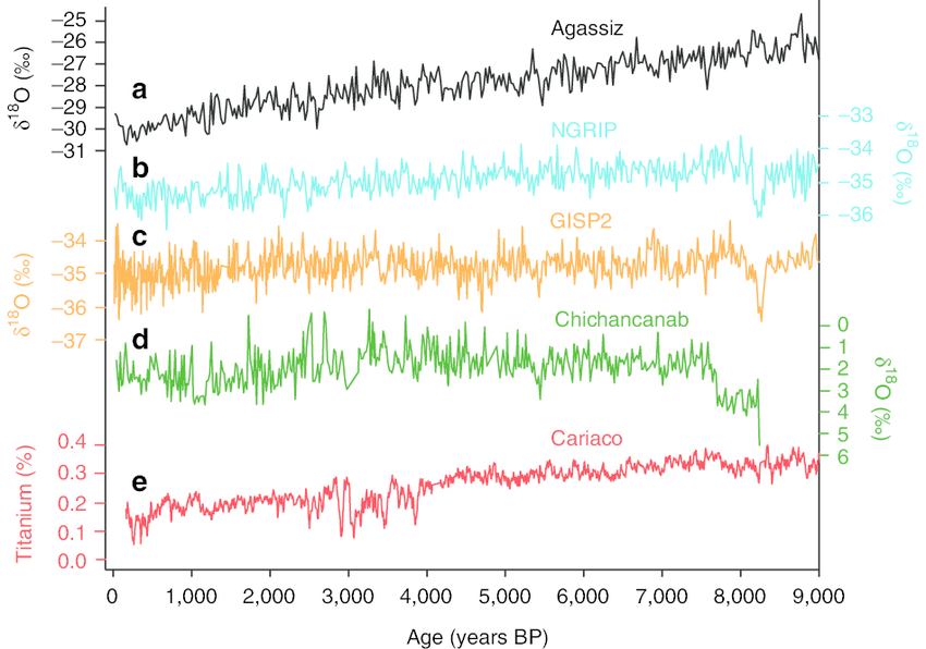
Below is data from Dome C, Antarctica, that provides a climate record for the past 740,000 years. For the four most recent glacial cycles, the data agree well with the record from Vostok (which only goes back 400k). The earlier period, between 740,000 and 430,000 years ago, was characterized by less pronounced warmth in interglacial periods in Antarctica, but a higher proportion of each cycle was spent in the warm mode. Note the difference between uncorrected ice core data from Volstok or Dome C, vs. corrected data.
NOTE HOW THE CORE DATA DOES NOT AT ALL AGREE WITH THE SEDIMENT RECORD OF TERRESTRIAL GLACIAL TILL. WE see three main glaciations in the sediment record going back 700k, but we see at least 7 in the marine isotope and ice core data. Why is that??? Neither of these can be directly dated well. I think the dates are WRONG. Core data is showing 3000 year TPW/expansion events. (where supposed 900k shows about 50 events suggesting its actually 150,000 years, NOT 1 million/900k years)
NOTE ALSO… the marine isotope data in the graphs above is pretty consistent with mostly equal peaks all the way from present to 2 million years ago. COMPARE THAT to the ice core data which shows these MASSIVE peaks at the 100k/40k Milankovitch cycle spots where they want ice ages. IN MY OPINION, THE DEAP SEA CORES ARE FAR MORE RELIABLE. ICE CORE DATA IS GARBAGE. It is too dependent on snow fall which is just not consistent.
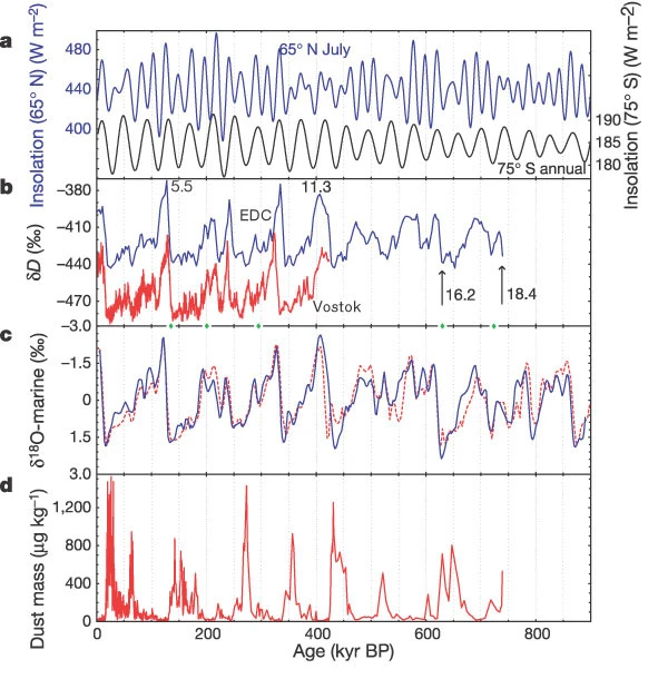
Comparison of EPICA Dome C data with other palaeoclimatic records. a, Insolation records4. Upper blue curve (left axis), mid-July insolation at 65° N; lower black curve (right axis), annual mean insolation at 75°S, the latitude of Dome C. b, δD from EPICA Dome C (3,000-yr averages). Vostok δD (red) is shown for comparison1 and some MIS stage numbers are indicated; the locations of the control windows (below 800-m depth) used to make the timescale are shown as diamonds on the x axis. c, Marine oxygen isotope record. The solid blue line is the tuned low-latitude stack of site MD900963 and ODP6773; to indicate the uncertainties in the marine records we also show (dashed red line) another record, which is a stack of seven sites for the last 400 kyr but consisting only of ODP site 677 for the earlier period2.
.
This needs to go earlier in the paper. Explain how it came to me and what it means for the disaster cycle and our new dating methodology.
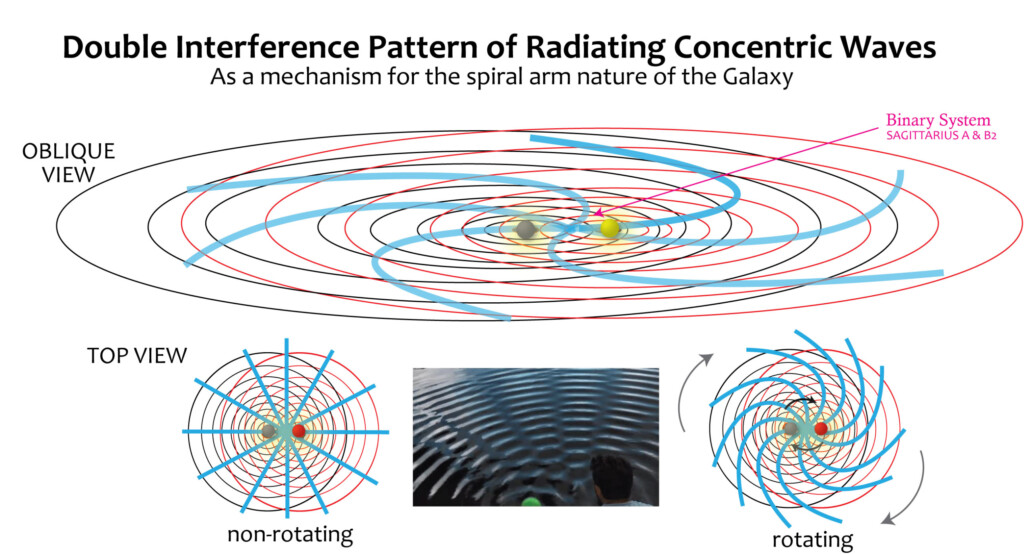
A Synthesis of Binary Galactic Dynamo Theory and Magnetohydrodynamic Resonance – A Galactic Double Interference Pattern of Radiating Concentric Waves
Important Background Concepts:
–Magnetohydrodynamics
–Magnetosonic Waves
–Alfvén Waves
–Galactic Density Wave Theory
The structural and electrodynamic architecture of the Milky Way galaxy suggests a governing mechanism far more complex than a simple monocentric gravitational well. While the presence of the supermassive black hole Sagittarius A* (Sgr A*) is well-established, the emergent morphology of the galactic disk—specifically its spiral density waves and the recently mapped radial magnetic filaments—points toward a Hierarchical Magnetohydrodynamic (MHD) Dynamo influenced by past merger events. This theory proposes that the galactic core has undergone transient dual-offset phases, where the interplay of merging centers of mass and energy generated complex, radiating interference patterns that scale fractally from the galactic nucleus to the local interstellar environment of our solar system.
The Hierarchical Engine and Spacetime Modulation
At the heart of this model lies a historical barycentric offset within the galactic core, potentially resulting from a recoiling black hole following a merger event with smaller galaxies or their black holes approximately 1-10 million years ago, or from gravitational coupling during such assimilations. In classical orbital mechanics, a single mass produces a static potential; however, a transient offset or merger-induced asymmetry functions as a rotational dipole during the dynamical phase. This dipole acts as a “paddle” in the galactic plasma, creating interference patterns analogous to oscillating sources in a fluid medium.
As these offset centers interacted during the merger, they emitted periodic pulses of gravitational-wave energy and, more critically, magnetosonic perturbations. These waves propagated outward through the Interstellar Medium (ISM). Where the wave fronts from the merging dynamics intersected, they created zones of constructive interference, manifesting as the high-density “spokes” or “spines” that seeded the primary spiral arms. This aligns with and expands upon Galactic Density Wave Theory, suggesting that the spiral arms originated as perturbation-induced wave fronts that evolved into stationary wave structures through which stars and gas periodically pass.
The Galactic Current Sheet and MHD Filament Radiation
Transitioning from gravity to electromagnetism, this merger-driven oscillation is mirrored in the galaxy’s plasma environment. The rotational asymmetry during the merger twisted the galactic magnetic field into a massive, three-dimensional Galactic Current Sheet. While the Sun’s heliospheric current sheet is often likened to a “ballerina’s skirt,” the Galactic Current Sheet, influenced by hierarchical dynamo processes, takes on a more complex, harmonic fluted shape. This sheet provides the structural foundation for the “spires” or filaments observed in the radio spectrum.
The radial filaments pointing away from Sagittarius A are interpreted here as Alfvén wave conduits—plasma “spires” radiating along the lines of magnetic flux. Because of the binary nature of the source, these spires are not uniform. They are subject to Mode Coupling, where different frequencies of magnetic oscillation overlap to create “sunburst” patterns of canceling and reinforcing waves. This interference creates a “fine structure” within the galaxy—a lattice of magnetic and density fluctuations that permeate the disk.
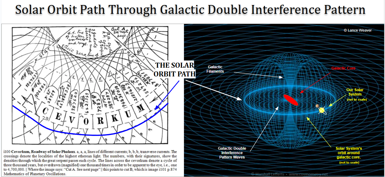
Fractal Periodicity and Local Interstellar Interaction
The most profound implication of this theory is the existence of fractal wave-levels rooted in ISM turbulence. Just as large-scale waves shaped the spiral arms over millions of years, smaller-scale, higher-frequency harmonics cascade through the galactic medium via self-similar turbulent processes. Our solar system, in its 230-million-year journey around the center, does not move through a vacuum but rather encounters these diffused filaments of plasma and compressed magnetic flux, potentially following periodicities observed in ice cores, climate data, and astronomical records, such as alignments with ~735/1,470/2,940-year cycles that could be tested against Berillium10/Carbon14 data.
The effects of these intersections are seen in the cyclicities of phenomena such as Dansgaard–Oeschger events, Bond Events, and Heinrich events, as well as carbon-14 and beryllium-10 evidence in Bray or Hallstatt cycles, though these are cautiously linked to solar dynamo modes amplified by inter-stellar-medium encounters rather than direct galactic wavefronts. On a galactic scale, the Hierarchical Magnetohydrodynamic (MHD) Dynamo manifests as the spiral arms of the galaxy itself. Secondary and higher-order harmonics create the “spurs” and “feathers” between arms (distanced hundreds of thousands of years apart), with smallest-scale fractal-based harmonics spanning an average of 735/1,470/2,940 years apart. These may in part explain what the MeerKAT radio telescope reveals in the ‘Bent Harp’ parallel Harp Cluster filaments, with a possible PTA ‘Red Noise’ or ‘Birkeland Current’ connection tied to merger-induced gravitational wave backgrounds.
This binary-driven MHD model provides a unified framework for understanding the Milky Way as a coherent, self-organizing system. By viewing the galactic center as a dual-oscillator, we can account for the misalignment of Sagittarius A’s spin, the existence of both radial and vertical magnetic filaments, and the periodic density fluctuations experienced by our planet. In this view, the galaxy is a resonant chamber, where the fundamental “hum” of the core is transmitted via plasma waves to the furthest reaches of the spiral arms, dictating the rhythm of stellar and planetary evolution.
The Magnetic Torque Mechanism of Pole Shift
The most plausible geomagnetic mechanism for pole shift involves the interaction of the planet’s magnetic field with the external plasma environment (the solar wind).
A. Solar Wind Interaction
- Magnetospheric Drag: A planet with a strong magnetic field (like Earth) creates a large protective bubble called the magnetosphere. The constantly flowing, charged particles of the solar wind impact this magnetosphere, but they do not hit the solid planet. Instead, the momentum transfer from the solar wind onto the magnetic field lines creates a small, continuous drag, or torque.
- Torque on the Magnetic Field: This torque acts upon the magnetic field structure that is rooted in the Earth’s liquid outer core. Because the magnetic field is generated by the moving fluid of the outer core, the torque is primarily applied to the core itself.
- Core-Mantle Coupling: The core and mantle are coupled with each other electromagnetically and gravitationally. Any torque on the core is therefore transferred to the mantle and crust, very slightly slowing the rotation of the planet as a whole–beginning in the outer core. This is a subtle effect, but it exists. (which slowing has currently accelerated as our magnetic field weakens)
B. Mechanism of Disruption: “Magnetic Quenching”
- MHD Breaking: The magnetosonic shock waves (MHD waves) induce a Lorentz Force that drags, offsets & disrupts the Coriolis Force driving the geodynamo of the liquid iron outer core.
- The Angular Conflict: The Earth’s internal field is roughly aligned with its rotational axis (Dipolar). If an external galactic field hits at a 60° tilt (the angle of the solar system to the galactic plane), it tries to “realign” the field lines in the upper layers of the core.
- The “Back-Reaction” (Lorentz Force): This external field creates a force that opposes the helical motion of the liquid iron. In MHD terms, this is called Quenching. By disrupting the “twist” (the alpha-effect) of the iron columns, the ripple effectively “shorts out” the dynamo generator.
- Weakening via Turbulence: The clash between the internal and external fields creates MHD Turbulence at the Core-Mantle Boundary (CMB). Instead of smooth, organized flow that creates a strong dipole, the flow becomes chaotic, causing the dipole to collapse into a weaker “multipolar” state (many small north/south poles instead of one big one).
Stage 1: The Magnetic Torque Catastrophe from MHD Breaking
- Geodynamo Instability: A geomagnetic reversal is initiated by highly turbulent and chaotic fluid motion within the liquid iron outer core. I hypothesize that these disrupting fluid motions are caused by changes to the Solar magnetic field induced by a passing galactic magnetosonic ripple (MHD waves). As this highly charged dust-filled ripple passes through the Solar System, the earth’s magnetic field weakens dramatically (as seen historically from cyclicity in paleomagnetism records).
- Hypothesized Torque: I hypothesize that the intense, asymmetric motion of the highly conductive liquid iron, combined with the extreme drop in field strength, creates an unusually strong and asymmetrical electromagnetic torque on the outer core.
- Angular Momentum Transfer: This powerful torque slightly changes the outer core’s angular velocity and transfers that momentum imbalance to the rigid, overlying mantle through electromagnetic and viscous coupling at the Core-Mantle Boundary (CMB).
Stage 2: Core Material Migration (The Destabilizing Mass)
This is the most speculative step, relying on an established connection between the core and the surface:
- Existing Conduits: We assume that mantle plumes (the source of hot spots like Hawaii or the flood basalts) are not just hot rock, but are connected to deep-seated structures. I hypothesize that the plume conduits—already routes of deep material transfer—are exacerbated or opened by the extreme pressure and temperature dynamics during the magnetic event. (The slight differential rotation between the core and mantle causes melting of lower mantle rock, and ‘freezing’ or condensing of outer core material with associated state change and radical expansion of of core liquid as it congeals into lower mantle horizons.)
- Liquid Iron Leakage: The immense pressure and energy unleashed by the chaotic outer core motion forces pockets of superheated, liquid iron alloy—the outer core material—to follow these open rising plume conduits, such as the mid oceanic ridges, into the lower mantle.
- Mass Anomaly Formation: As this super-dense core material rises and mixes with the less-dense mantle, it would create subtle bulges and, new density anomalies high up in the mantle (perhaps just beneath the crust, like the formation of the Columbia River Basalts, only with iron-rich, hyper-dense material).
Stage 3: The Rapid True Polar Wander (TPW) Event
- Inertial Imbalance: The new, massive, and extremely dense concentration of core material high in the mantle represents an overwhelming rearrangement of Earth’s internal mass. This instantly shifts the planet’s principal axis of inertia away from its rotational axis.
- The Reorientation: The entire solid Earth (the crust and mantle) begins to rotate wholesale relative to its spin axis to bring this massive new anomaly closer to the equator, where it is most gravitationally stable.
- Magnitude and Speed: This change in the moment of inertia would be vastly larger than those caused by ice sheets or normal mantle convection. The resulting TPW event would be rapid (likely occurring over a few hundred thousand years or less—a geologic instant) and could easily shift the pole by thousands of kilometers (hundreds of miles), profoundly changing the geographic location of the North and South Poles relative to the continents.
While this mechanism is new and hypothetical, rapid, large-scale True Polar Wander events are supported by the consensus of geological evidence in the past:
- Cambrian TPW: The most debated and largest proposed event is the Early Cambrian Inertial Interchange TPW event (~ 530-500 million years ago), which suggests the Earth’s solid surface rotated by up to 90 degrees.
- Late Jurassic Shift: Paleomagnetic data also support a proposed “monster shift” during the Late Jurassic (~ 160-145 million years ago) involving a total rotation of ~30 degrees over about 12 million years.
These past events show that Earth’s crust and mantle can and do reorient rapidly (geologically speaking) in response to large internal mass changes.
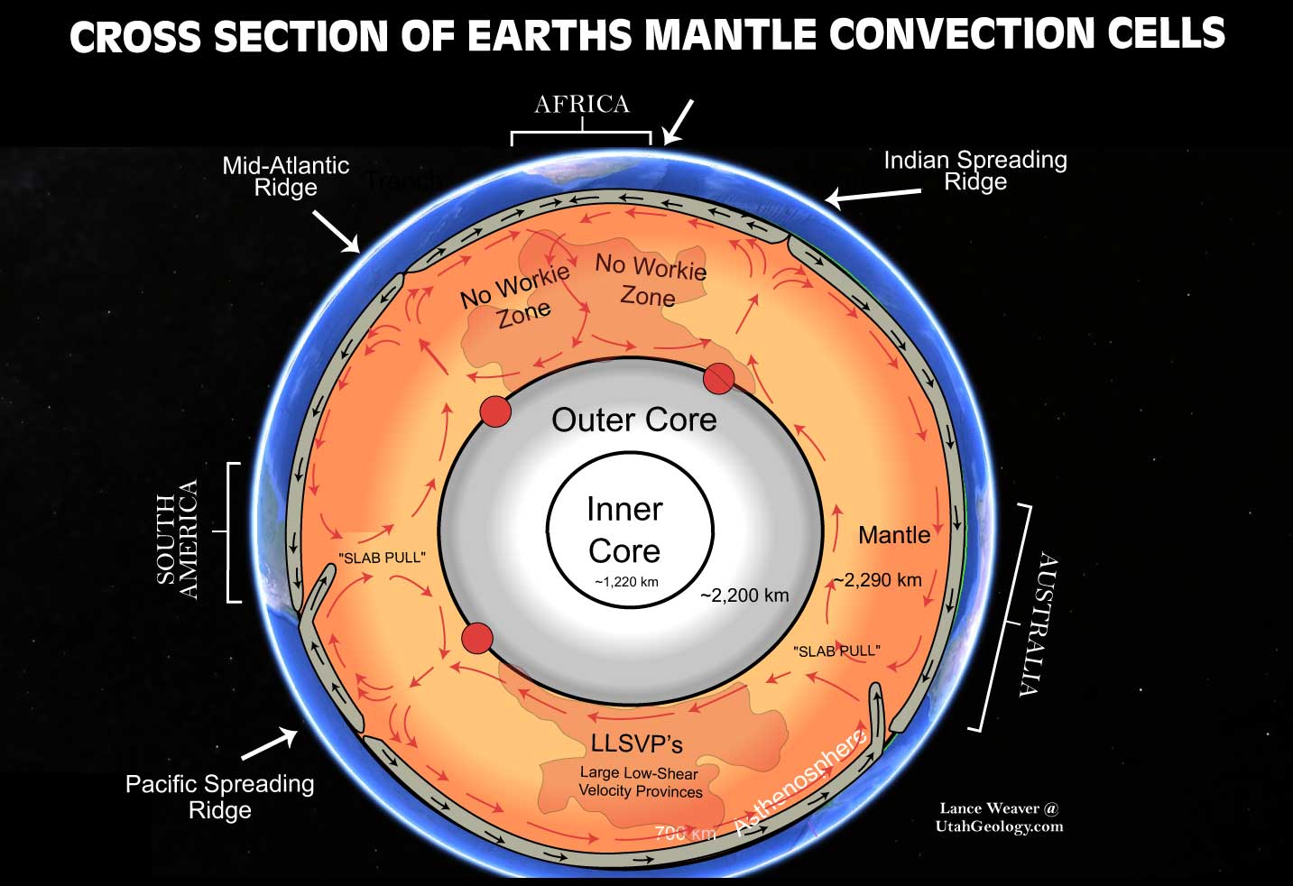
LLSVPs as Expanding Core-Mantle Composites
This theory posits that Large Low-Velocity-Shear Provinces (LLSVPs) are not accumulated mantle material but rather massive, thermally and chemically altered structures composed of core-material remnants that were stabilized and forced upward by a catastrophic (and expansive) phase change.
Stage 1: The Core-Mantle Boundary (CMB) Incubation
This stage requires an extreme, localized interaction at the CMB to create a chemically stable, non-sinking intermediary material.
- Chemical Erosion Pockets: Instead of simple thermal conduction, the chaotic flow of the liquid outer core causes intense chemical erosion of the silicate lower mantle at localized “hotspots” or trenches at the CMB. This process creates dense pockets of a new, hybrid material known as core-mantle alloy (or “protolithic” material).
- Iron-Silicate Solution: This core-mantle alloy is a super-dense solution of liquid iron and highly dissolved silicate rock, existing at the extreme pressures and temperatures of the CMB. This solution acts as a transitional layer, slightly less dense than the pure outer core but still significantly denser than the normal lower mantle.
- Phase Boundary Pinning: These pockets become pinned to the CMB by slight topological features or the flow geometry of the outer core. Over vast periods (hundreds of millions of years), they grow massive through continuous core-mantle interaction.
Stage 2: Catastrophic Pressure Release and Phase Expansion
This is the core mechanism that causes the material to overcome buoyancy and rise dramatically.
- Galactic or Solar Forcing Event: An extreme, outside-driven event (galactic wave fronts explained elsewhere in this paper causing magnetic or rotational chaos) creates an immense localized pressure wave at the CMB, disrupting the stability of the pinned core-mantle alloy.
- The Pressure Threshold: This pressure wave forces a section of the core-mantle alloy into a slightly higher-pressure region of the lower mantle, crossing a critical phase boundary for this new hybrid material.
- The “Freeze-Boil” Expansion: At the lower pressure of the mid-mantle, the core-mantle alloy undergoes a radical and rapid phase change (analogous to a “freeze-boil” event):
- The dissolved silicate components crystallize instantly into a rigid, low-density mantle structure.
- The iron component, now isolated from its silicate solution partner and no longer under core pressure, experiences a dramatic volume expansion as its crystal structure shifts into a metastable, less-dense form (e.g., a highly porous or “fluffy” metal phase not stable under normal core pressures).
- Creation of the Massive Anomaly: The combination of crystallization and volume expansion instantly transforms the super-dense core-mantle alloy pocket into a massive, warm, and highly buoyant (low-density) structure—the LLSVP. This rapid expansion provides the non-buoyancy-driven force to lift the material into the mid-mantle.
Stage 3: Stabilization and Anchoring of the LLSVP
- LLSVPs as Thermal Plume Sources: The newly created, buoyant mass immediately begins its ascent. Because it originated from the core boundary, it is extremely hot. This heat source provides the energy to drive thermal upwellings—the mantle plumes—which stream off the LLSVP and toward the surface (e.g., Spreading ridges/ Hot-spots like Hawaii, Iceland).
- Thermo-Chemical Anchoring: The “fluffy” or porous nature of the expanded core-material component gives the LLSVP its stable, low-shear-velocity seismic signature (S-waves slow down due to the anomalous structure). Although rising, its total chemical composition remains heavier than the surrounding pure mantle rock, keeping the base of the LLSVP “anchored” to the core boundary, even as the rest of the structure balloons upward into the mantle.
In this model, the LLSVPs are the result of a catastrophic, expansionary phase change of a super-dense, hybrid core-mantle alloy that was only possible due to extreme, time-dependent pressure dynamics at the CMB.
Climate Evidence for a 735 / 1,470 / 3,000 year MHD Oscillations.
1300 AD – Little Ice Age (LIA), and Plague cycle. (1346-1353ad)
550 AD – Late Antique Little Ice Age (LALIA), and Justinian Plague (541-549ad)
185 BC – Roman Warm Period (opposite period)
920 BC – Levantine Iron Age Anomaly (LIAA) between 1050-700bc
Questions & Answers:
-What’s this explain? The earth’s temperature anomalies and TPW disaster cycle.
-What causes these cycles? Large magnetosonic ripple or MTD waves emanating out from the Galactic core.
-What is their frequency? 35 / 1,470 / 3,000 years
-How do they cause temperature anomalies and TPW? By affecting both the solar & planetary dynamos. These plasma waves carry a charge density. These cause extremes in the Solar cycles with more violent maxima and a more depleted field during the minima…. finish… but the main effect to the earth actually happens during solar minimum when the solar electromagnetic field drops to a minimum and we are exposed to the galactic field for a prolonged period…. This creates a drag on the outer core, slowing it, and disrupting the dynamo… which can then completely fail or simply partially reorganize in an excursion. Either way, the drag disruption causes HEAT from both the induced current (Lorentz force) and the increased friction between the core & mantle which causes melting and PHASE CHANGE of core fluids as they are driven into the mantle, which causes expansion, which causes mass imbalance which often causes a wobble.
.
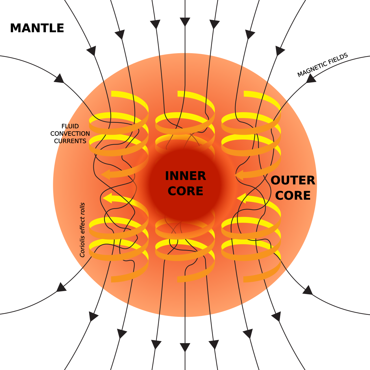
.
.
GeoMagnetic Reversals
So what causes reversals? This quote and following AI commentary might be the best explanation out there. It has to do with the magnetic pole approaching the geographic pole (during a 3k/excursion event I believe). When that happens it’s almost like two positive poles to a magnet approaching each other, they suddenly repel. So as the magnetic and geographic poles approach, the spin of the inner core tangles the deep magnetic lines. This tangling saps the power of the main magnetic field and creates a powerful magnetic “whirlpool” that rapidly snaps the magnetic poles together, zeroing out the field.
To answer this, under the project control of Dr. Paul A. Siple, the Rand Corporation was contracted to conduct lab studies using models of the earth constructed of concentric spheres – an inner sphere representing the electromagnetically-charged molten iron core of the earth whose axis defined the ‘magnetic’ poles; and an outer sphere representing the crust of the earth which rotated around a ‘geographic’ polar axis. It was determined through repeated experimentation that as the ‘magnetic’ pole approached the ‘geographic’ pole, the ‘magnetic’ pole would at some point accelerate its rate of convergence as though pulled toward the ‘geographic’ pole by centripetal force and jump to coincide; but instead of the poles coinciding, the ‘magnetic’ pole would rapidly ‘flip’ around the ‘geographic’ pole, then spin off towards the equator as though by centrifugal force, ending up at a position where the two axes assumed an approximate 89-degree divergence. After this polar ‘flip’ occurred, the axes would then gradually begin to reconverge over a long period of time.”
SO NOTE. Reversals dont happen every 3k period, only when the cycle happens to end when poles are converged.
The Rand Corporation’s Concentric Spheres Model and Related Geomagnetic Experiments
AI: The quote you provided describes a specific mid-20th-century modeling effort to simulate geomagnetic pole behavior, often cited in discussions of Earth’s magnetic field dynamics and potential “pole shifts.” I’ll break this down with historical context, verification of the experiment, similar subsequent work, and the prevailing scientific theories explaining the observed “flip” behavior in such models. This draws from paleomagnetic and geodynamo research, where physical analogs help test hypotheses about Earth’s core.
The Original Experiment: Rand Corporation’s Model Under Paul Siple (Late 1940s–Early 1950s)
The described setup aligns with a classified U.S. military-sponsored project led by Antarctic explorer and geophysicist Dr. Paul A. Siple (1908–1968), who served as a scientific advisor to Admiral Richard E. Byrd and contributed to early Cold War-era geomagnetic studies. Siple’s work focused on polar exploration and magnetic variations, motivated by concerns over rapid shifts in the North Magnetic Pole (observed accelerating toward the Geographic North Pole post-WWII, raising navigation risks for aviation and submarines).
- Project Details: In the late 1940s, under Pentagon discussions (attended by figures like Major H.A. White), the Rand Corporation (a think tank contracted for defense research) built physical analogs to predict what happens when magnetic and geographic poles converge. The model used concentric spheres:
- Inner sphere: A magnetized core (simulating Earth’s electromagnetically charged molten iron outer core), with its axis defining the “magnetic poles.”
- Outer sphere: A non-magnetic shell (representing the crust), rotated independently around a fixed “geographic” polar axis.
- Experiments involved gradually aligning the spheres’ axes (mimicking pole drift) using controlled rotation and electromagnetic induction.
- Observed Behavior: As the magnetic axis approached the geographic one (within ~1–2 degrees), the inner sphere’s field destabilized, causing the magnetic pole to “accelerate” (via induced torque), “flip” around the geographic pole (reversing polarity), and then diverge to ~89° (nearly equatorial). This reconverged slowly over simulated “cycles.”
- Purpose and Outcome: The goal was to assess risks of a “polar flip” (not a full crustal displacement, but field instability). Results suggested a rapid, oscillatory reversal rather than stable coincidence, published in declassified reports around 1950–1953. Siple’s involvement stemmed from his 1946–1948 Arctic expeditions tracking pole movement (e.g., via Air Force Reconnaissance Squadron data, declassified in 1988).
- Sources and Verification: This is detailed in Charles Hapgood’s The Path of the Pole (1970, revised 1991), drawing from Siple’s memos and Rand’s internal papers. Primary refs include Siple’s 90° South (1959) and Rand’s geomagnetic surveys (e.g., 1952 reports on pole wander). No full public dataset exists due to classification, but it’s corroborated in declassified U.S. Navy geomagnetic archives. Skeptics note Hapgood’s fringe interpretations (e.g., linking to cataclysmic crustal shifts), but the core model is legitimate 1950s analog research.
Similar Experiments Since the 1950s
Post-Rand, geodynamo modeling evolved from simple mechanical analogs to sophisticated fluid dynamics simulations, driven by computing advances and the need to explain paleomagnetic reversals (Earth’s field has flipped ~183 times in 83 million years). Key examples:
- 1960s–1970s: Early Computer Simulations (Glatzmaier-Roberts Model): Robert Glatzmaier and Paul Roberts developed numerical models of concentric spheres with convecting fluid (molten iron analog) in the outer shell. Their 1995 simulation (published in Nature) reproduced spontaneous pole flips over 40,000 simulated years, matching the Rand “flip” but attributing it to turbulent flow instabilities. This became foundational for dynamo theory.
- 1990s–2000s: VKS Experiment (France): At the Grenoble Observatory, the VKS dynamo experiment used two concentric spheres filled with liquid sodium (conducting fluid mimicking the core). The inner sphere rotated at variable speeds, inducing a self-sustaining magnetic field that reversed polarity irregularly—observing ~10 flips in lab time, with poles “jumping” due to helical flow patterns. Published in Physical Review Letters (2006), it validated the Rand-like divergence to ~80–90° before reconvergence.
- 2000s–Present: Lathrop’s Sodium Spheres (University of Maryland): Daniel Lathrop’s team built a 3m-diameter setup with an inner sphere (1m, spinning at 960 RPM) inside 13.5 tons of liquid sodium (outer sphere at 240 RPM). This 2010s experiment simulated 5,000 Earth years per second, producing chaotic fields with multiple poles and flips (e.g., 180° reversals in hours of lab time). It showed “centrifugal-like” ejections to equatorial zones, echoing the Rand model’s 89° divergence. Funded by NSF, results appear in Geophysical Research Letters (2013–2020).
- Recent Advances (2020s): Numerical models like those from Andrew Jackson (University of Leeds) use supercomputers to simulate 3D turbulent dynamos, reproducing flips in concentric setups with added core-mantle boundary asymmetries. The 2020 World Magnetic Model update incorporated such data to track real-time pole drift.
These build on Rand by using fluids (sodium/mercury) for realistic dynamo effects, rather than static magnets.
Prevailing Theory: Why the “Flip” and Divergence Occur in Concentric Rotating Magnetized Spheres
The behavior in the Rand model (and successors) isn’t a literal “centripetal/centrifugal force” pulling the pole but emerges from geodynamo instability in rotating, conducting fluids. The prevailing explanation, rooted in dynamo theory (developed by Joseph Larmor in 1919, refined since the 1950s), is:
- Mechanism: Earth’s magnetic field arises from the geodynamo—convection in the liquid outer core (molten iron-nickel alloy) driven by heat from the inner core and mantle. Rotation (Coriolis effect) organizes helical flows, generating electric currents that sustain the field via electromagnetic induction.
- Why Convergence Accelerates: As axes near alignment (~1–2° apart), the field’s dipole weakens due to toroidal-poloidal coupling. The rotating inner sphere’s field lines twist (like a solenoid), amplifying torque near coincidence, “pulling” the pole faster via induced eddy currents—simulating centripetal attraction.
- The “Flip” and Ejection: At minimum separation, the system hits a bifurcation point (instability threshold). Turbulent eddies and alpha-omega dynamo effects cause chaotic reconnection of field lines, flipping polarity (north↔south). Instead of stabilizing, angular momentum conservation “flings” the new pole equatorward (centrifugal analogy), reaching ~89° divergence as the field multipolarizes (multiple temporary poles form). This matches lab observations where low field intensity (~10% of normal) allows non-dipole states to dominate briefly.
- Reconvergence: Over “long” times (thousands of simulated years), viscous drag and Coriolis forces realign the dipole along the rotation axis, restoring stability. In real Earth, this takes 1,000–10,000 years per reversal.
This is supported by paleomagnetic data (e.g., seafloor stripes from Vine-Matthews hypothesis, 1963) and simulations showing reversals as random, non-periodic events (~every 200,000–300,000 years). No evidence links i
NOTE THAT THE LAW OF ONE TALKS ABOUT THE ‘EXPANSIVE CONSEQUENCES OF HEAT’ (that can’t correctly escape the earth’s system.) This suggests that each 3000 year cycle, something has been happening to heat the earth, so its not cooling over time, its heating. Which doesn’t make sense when you think how much hotter the earth’s atmosphere was in the Mesozoic, but apparently something has happened so internal heat & gas gets trapped since the Cretaceous.
Due to the nature of the physical vehicle, disharmony shows up as a blockage of growth or an uncontrolled growth since the primary function of a mind/body/spirit complex’s bodily complex is growth and maintenance. In the case of your planet the purpose of the planet is the maintenance of orbit and the proper location or orientation with regards to other cosmic influences. In order to have this occurring properly the interior of your sphere is hot in your physical terms. Thus instead of uncontrolled growth you begin to experience uncontrolled heat and its expansive consequences.
Perhaps one possibility is the ‘freezing’ effect talked about in the below video where outer core liquid is ‘freezing’ or solidifying/quagulating onto the inner core, expanding it. But more likely there is some aspect of the interior of the earth that we have wrong and is GREATLY expanding over time as it is heated by radioactive decay of the core. (perhaps the lower mantle?)
Remember that I did the math on how volcanic plumes expand hundreds of times in size as they expand to the surface. Something similiar to this must be happening, perhaps as massive plumes of magma rise to fill the mid oceanic ridges, which then expands more and fuels more rifting? Another theory is that our core has something like the process of star swelling that happens in Red Giants when nuclear fusion ceases in the core, causing it to contract and heat up. This heat ignites a shell of fusion around the core. This enormous release of energy pushes the outer layers of the star dramatically outward.
.
Overview:
https://www.nature.com/articles/s41598-022-11493-1/figures/1
https://www.nature.com/articles/s41598-022-11493-1
Raw Data:
https://www.researchgate.net/publication/331398373_Seawater_Temperature_and_Dissolved_Oxygen_over_the_Past_500_Million_Years/figures?lo=1
https://www.researchgate.net/publication/331398373_Seawater_Temperature_and_Dissolved_Oxygen_over_the_Past_500_Million_Years
-This precession is the primary cause of plate movement and true polar wander
-True polar wander is (define)
-Its a lot like the X principle of a top, or the Y principle of an atom in an electric field.
-The precession was likely begun and periodically altered by a combination of bolide impacts and electric field variations.
-random bolide impacts and changes in the solar and galactic field strength change our processional amplitude and timing
-The Oxygen isotope variations we see in Pliocene and Pleistocene have been misinterpreted at glacial cycles. They are not! The differences seen in pre-Pliocene vs post-Pliocene oxygen18 swings has to do with older/deeper material being compressed to a degree that flattens the curve. Show how summer/winter variations or secular variation like we’ve seen in the last 2000 years match the variation we see in the Pleistocene.
.
Compare these:
https://www.nature.com/articles/s41598-022-11493-1
https://www.science.org/doi/10.1126/science.1221294
To these: !!!! (make an illustration of this!!
https://www.sciencedirect.com/science/article/pii/S0277379122005613
https://www.sciencedirect.com/science/article/pii/S0277379122005613#fig5
https://www.ncbi.nlm.nih.gov/pmc/articles/PMC7614327/
(find a better one from more like 7000 BP to present. Or 20,000 BP to present.
TODO: Put the pole locations at different ages on this image as well as making an outline of North America and showing it move away from Europe and explain how ice age starts when the opening begins, and that the pole hasn’t drifted north hardly at all since 20mya, its just moved mostly west with North America. Show another location with the plate ages and more importantly, the Greenland Transverse Fault (which matches with the San Andréa’s Fault (starting 35-28 million years ago) but really accelerating with the swallowing of the Farallon plate/spreading ridge 20mya (draw spreading ridges on this image!)
-Add a graph showing the likely velocity of change for the pole shift. For instance, if it averaged 0.5 mph then it would take 2000 hours or 83 days to happen. I’m proposing something closer to 200 years. Which would be a speed of 0.00058 mph basically inperceptable.
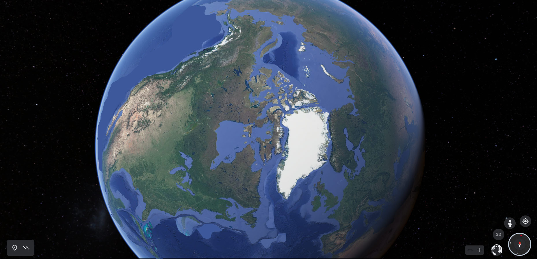
.
.
Abstract: Variable Speed of Light as a Mechanism for Apparent Radioactive Age Inflation
A speculative cosmological model proposes that the speed of light (c) was significantly higher in the early universe, decreasing over cosmic time as the universe expanded. This variable speed of light (VSL) framework, inspired by theories addressing the horizon and flatness problems without inflation, suggests that nuclear decay rates—governed by fundamental constants involving c—were correspondingly faster in the past. As c slowed to its present value, decay rates decelerated, causing radiometric clocks to accumulate daughter isotopes rapidly early on while running slower later. Consequently, geological samples formed billions of years ago would exhibit inflated apparent ages when measured with modern decay constants, potentially compressing a true 20-million-year history into dates exceeding a billion years.
This mechanism avoids catastrophic heat or radiation excesses associated with accelerated decay models by rescaling physical units with c, preserving energy conservation in a modified relativity framework. While offering a unified explanation for “old-looking” young rocks without ad-hoc divine intervention, the theory remains highly constrained by observational limits on historical variations in c and the fine-structure constant (Δc/c < 10⁻⁵–10⁻⁷ over cosmic time), rendering drastic million-fold changes incompatible with quasar spectra, CMB data, and Big Bang nucleosynthesis. Nonetheless, it represents one of the more physically coherent alternatives to constant-c cosmology for reconciling discrepant radiometric ages
Strengths (Why It’s “Believable” Among Alternatives)
- Solves cosmology issues (horizon, flatness) without exotic inflation fields.
- Tested variants predict altered CMB/black hole thermodynamics—falsifiable (e.g., fine-structure variations in quasar spectra constrain Δα/α < 10^{-5} over 10 Gyr).
- No divine intervention; pure physics.
Fatal Weaknesses
- Observational Constraints: Quasar absorption lines, CMB, and Big Bang nucleosynthesis limit |Δc/c| < 10^{-5}–10^{-7} over cosmic time—far too small for million-fold decay shifts.
- Lorentz Violation: Changing c breaks relativity; no evidence in particle accelerators or GPS.
- Heat/Radiation: Even mild VSL produces detectable energy mismatches.
- No Mechanism: What physical field drives c(t)? Proposals (scalar fields) are unconstrained/ad-hoc.
Thick Atmosphere Theory
This theory doesn’t hold up. First off, because dragonflies and bees would not have been able to evolve with their delicate wings in the Paleozoic like they did. Its more likely that pterosaurs had wings and feathers like modern birds. Although debated there seems to be more and more evidence of this being found. And they weren’t really that big. The biggest full fossil found had a wing span of 8.5 feet. Smaller than a modern condor or albatross. Must have been temp that changed the density of the mantle NOT an ancient thick atmosphere.
UNDER CONSTRUCTION FROM THIS POINT ON:
— add a sat image of Scandinavia scour surface. add a pic of thermokarst and how it is NOT a glacial landform.
NEXT section. Title: The Catastrophism/Uniformitarianism Debate. The debate is well documented. Until the early 1900’s it was the predominate explanation for earth processes. However, with time uniformitarianism won out. Why? Because it did a better job of explaining observed phenomena. However, because deeply held religious beliefs were often involved the debate had a tendency to polarize individuals into extreme camps. Instead of looking objectively at evidence and creating models based solely on logic, many individuals felt that had to take an “all or nothing” approach to their chosen camp. Now that decades have gone by, and people have had a chance to disconnect themselves from the emotion of this debate, a more rational middle ground is emerging. Somewhat catastrophic events such as the asteroid impact hypothesized to have caused the dinosaur extinction or to have caused the Younger Dryas cooling event during the Ice Age are becoming mainstream. Articles on ancient rapid true polar wandering are sprinkled throughout the scientific literature.
I’ll finish this article when I have time. For now the rest is just notes.
-I have to admit that it’s kind of weird that while studying the solar zenith tube at Monte Alban and Babylonian alignments/correlations with the helical rising of the Shepherd, I had a nagging suspicion that the 49 days of Pentecost also are somehow related to the 49 days where the sun “stands still” or stays at its perceived zenith for those observing at the 21.7 latitude. (And note, Mecca is found nearly EXACTLY 21.7 degrees latitude). But it makes me suspect that Sanai or Jerusalem must have been at the 21.7 latitude before Moses for Pentecost to make the most sense. Which would mean the north pole has changed by some 700 miles since then. (And directly in the direction of Giza, since the pyramids still face nearly exactly north.. which would put the North Pole at Moses (just before Moses), at the location the above illustration and study shows it occupied at 30mya! Coincidence? Probably. It doesn’t really even make sense. But something to keep in mind.
TO DO:
-most true polar wandering events proven in the literature occur on timetables of at least a million years. To rationally suggest a rotational axis change of 25 degrees latitude within just a few thousand years will require not only a believable mechanism, but physical calculations about how this could be accomplished without tearing the earth apart or causing overwhelming catastrophe with the changes in angular momentum & inertia.
-talk about how this was a debate back in the 50’s and 60’s, especially with charles hapgood’s books (as well of velikovsky). But a believable mechanism for rapid pole shift was not conceived. Even though Einstein himself wrote the foreword to Hapgood’s book, and supported his theory that the weight of the ice itself destabilized the axis, the whole premise was too extreme, and smelled too much of biblical catastrophism for the scientific community to accept.
Talk about the comet impact theory for the Dryas Minima and how this combined with imbalances caused by the iceland mantle plume seem to some of the best explanations for a cause of the TPW

Paleomagnetic Reconstructions

Our current understanding of where pole is is based on several points of evidence….. POINT HERE NEEDS TO BE THAT RECONSTRUCTIONS ARE ONLY ACURATE TO 20 DEGREES, GIVES A GREAT BALLPARK FIGURE BUT HORRIBLE EXACT LOCATION. Be sure to reference this page, that shows how off CURRENT measurements are. http://all-geo.org/chris_rowan/2014/01/paleomagnetism-lab-testing-the-gad-hypothesis/
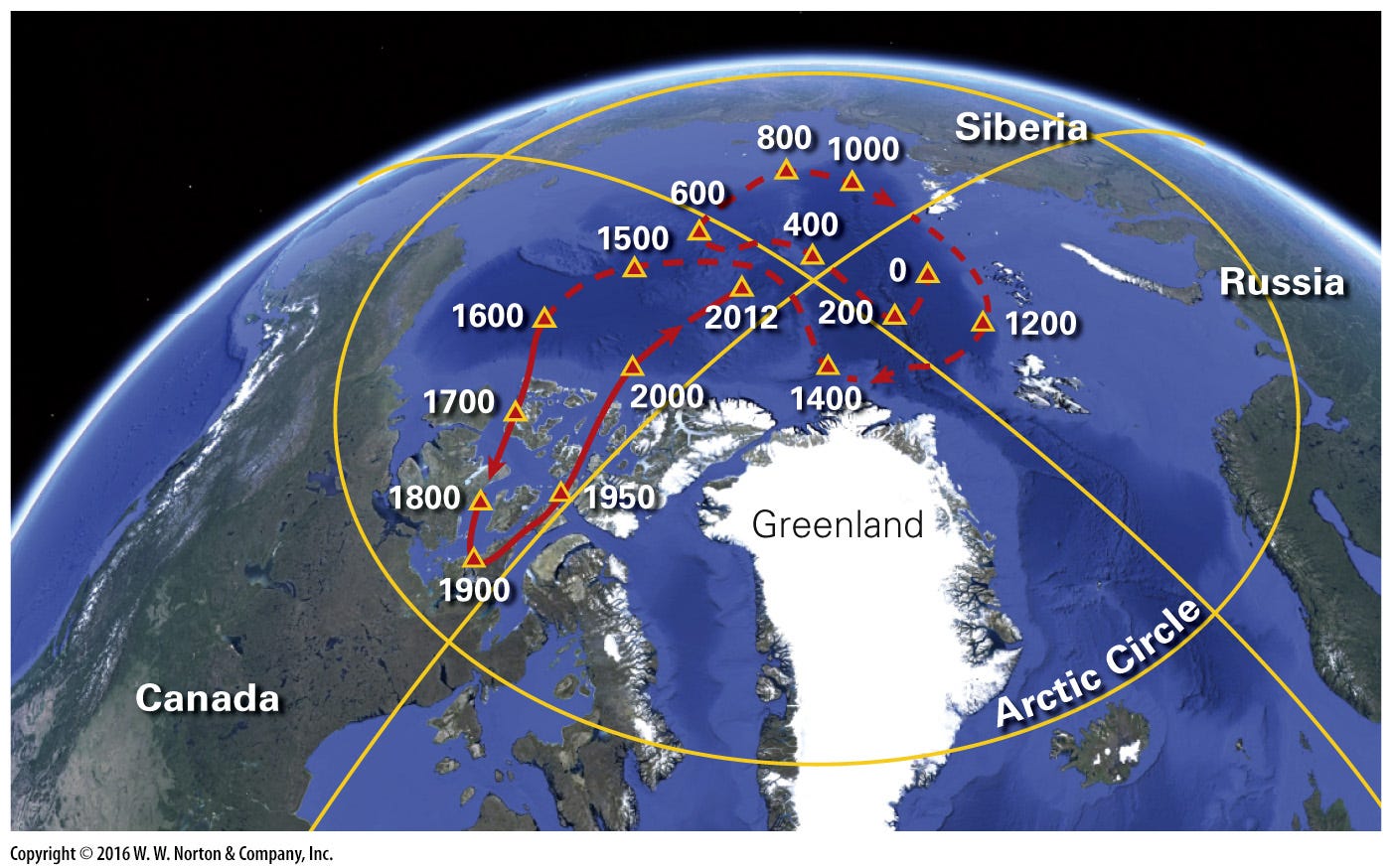
Possible Causes
Some are cyclical, some are random. Make an illustration showing the core slightly off center to show how earth would now wobble, and then stabilize over time.
- Gravitational effects of sun and Jupiter on moon and equatorial bulge (same things that cause precession-go into detail on how this is likely ALSO what creates the earth’s and suns magnetic fields, and same forces cause sun to flip and probably cause earth’s to flip too). There’s a good amount on the correlations between Jupiters 11 year orbit and the suns 11 year solar cycle (with Saturns gravitational effects causing the half year difference in timing). Note this important fact. The moon is NOT orbiting earth’s equatorial plane, its on the SUNS equatorial plane (2–5 deg off), so the combined tidal forces of the moon and sun pull earth’s core double and unevenly.
- Bolide/asteroid impacts. (this is a big one, partly random and partly cyclical because arms of galaxy hold more debris. The proposed impact for the younger dryas is a great possibility as one of many)
- Gravitational waves (also a big one, because it literally warps space time and compresses the earth longitudinally. can be both cyclical and random between those coming from center of galaxy and those caused by supernova). Reference my article on how these are responsible for the arms of our Galaxy, and how when we cross these waves every 4000 years or so, it cause slight wobble events. (which if there is enough built up instability triggers a TPW event).
-TPW “excursions” caused by “destabilization events”. The evidence for glaciation in Patagonia and Siberia is a huge problem. It seems to suggest that the pole must have gone from north of present to greenland and back! How is that possible? And it doesn’t match well with any polar wandering data (of course those kinds of anomolous data points are often thrown out of studies). And why is Antarctica’s glaciation so much older than the north hemisphere? South-East Antartica should have the oldest ice. North-East Antartica & the Penensula should have the youngest. Does this match with data? See evidence for each area’s glaciation here: http://www.science.earthjay.com/instruction/HSU/2015_fall/GEOL_553/literature_sources/ehlers_gibbard_2007_cenozoic_global_glaciation.pdf — — -this what you have to work with. So this idea solves it. THE CORE is more dense, it gets pulled by gravity more and destabilizes the earth. BUT the equatorial bulge resists the dif spin, causing mantle to differentially rotate (making the mag field by the way). but every 100,000 radiocarbon years or so the destabilization hits a tipping point and the SLOW TPW looses balance and the earth goes for a TPW trip. For the last 3 million K/Ar years this has been TOWARD the “North Atlantic gravity anomaly” (there also one north of Australia likely playing a part). And asteroid hitting the moon might just knock its orbit eccentric enough to affect tidal forces on the mantle.
Evidence Against Catastrophism
Be sure to add a whole section here on what I see in river systems and orogenic uplifting and folding on the Colorado Plateau. Its important to see the powerful evidence for uniformitarian orogenesis in earth’s river systems which traverse folded strata. For instance, even the smallest tributaries of the Colorado River cut through massive folds which obviously have risen slow enough over their evolution to avoid rerouting of the river systems. Only a few examples such as the Unaweap Canyon through the Uncompahgre Plateau show evidence of rapid enough uplift to reroute the river. This suggests to me that although these pole shirts are occurring fast in “geologic time”, they are not occurring fast enough to catastrophically reorganize plate motions.
Now this is where it gets crazy
Rapid polar wander events are fairly well documented and accepted in the Scientific literature. Just one of many examples is the Jan 2000 issue of Science which published evidence of “Late Cretaceous Polar Wander of the Pacific Plate: Evidence of a Rapid True Polar Wander Event“. These types of events are typically hypothesized to occur over about a million years. And of course debate will always exist as to whether these perceived rapid polar wandering events are simply movement of the magnetic pole, instead of true polar wandering of the rotational pole or axis (since in the geologic record it is difficult to tell the difference between the two). Debate also rages as to which reference system is the most reliable, as every continent and seamount system gives a different APW (apparent polar wandering) path since the plates all move separately from each other over time. However, to me the most interesting data point is the lack of Paleozoic strata under the entirety of the Pleistocene polar ice sheet! Where did it go? Are we to believe as some suggest that the entirety of the Canadian & Scandian Shields were above sea level for the last 500 million years in a configuration matching exactly with the ice sheet. That seems entirely impossible to me. Or are we to believe that the Pleistocene Ice Sheet removed/eroded essentially ALL Paleozoic strata? Although far more likely than the first possibility, this still seem unlikely to me. So then where did it go? When I see that the seamount reference frame shows an APW (apparent polar wandering) path matching closely with the location of the radiocarbon dated Pleistocene Ice Sheet it simply seems more likely to me that some type of ice sheet actually existed in that area for far longer than the Pleistocene. Perhaps more likely since the Eocene thermal maximum, when the Antarctic ice sheet is known to have began growing (or possible even into the supposedly “hot house” Cretaceous). Looking at the data, I cant get past the most obvious answer, that a Scandian & Canadian Ice Sheet existed in these “ice age” locations for much of the past 45-120 million years, and that this explains why there is essentially ZERO Paleozoic sediment in those locations. And that some kind of mechanism (likely a mantle plume) actually has had the rotational axis shifting back and forth from at least the end Eocene — causing along with it some type of overlap in radiometric dates. (
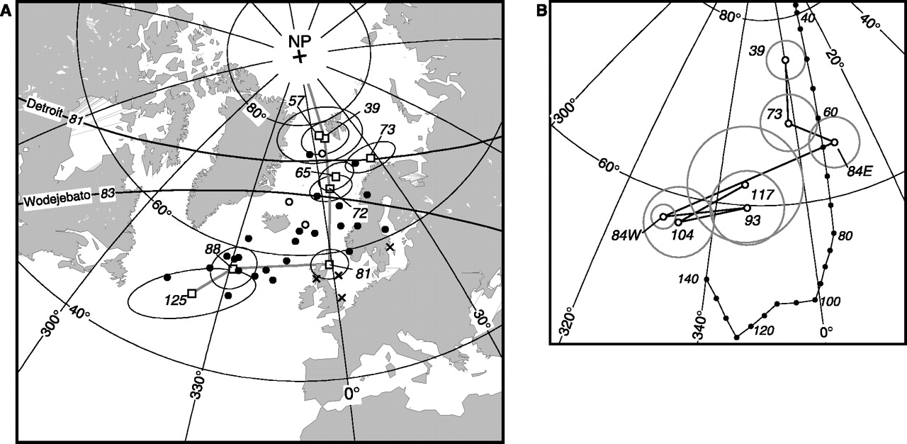
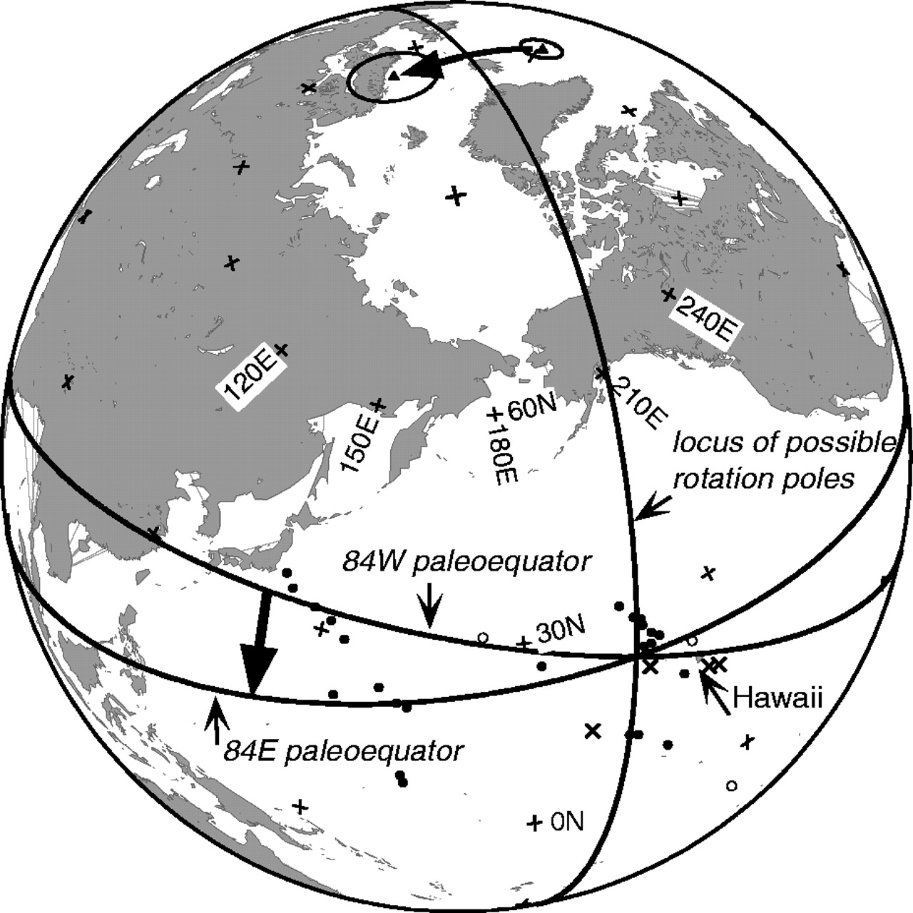

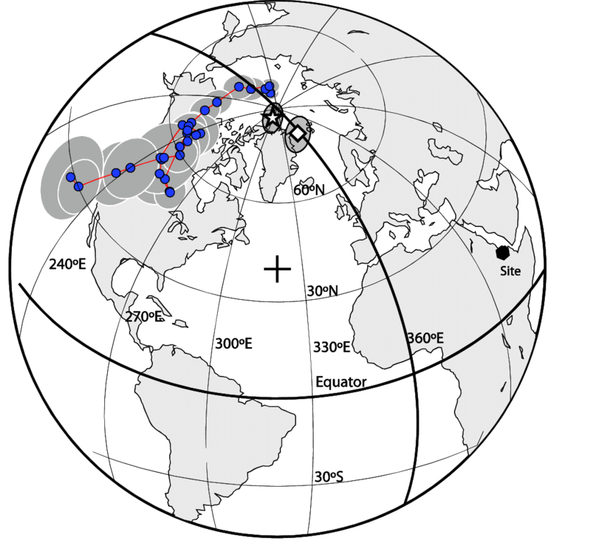
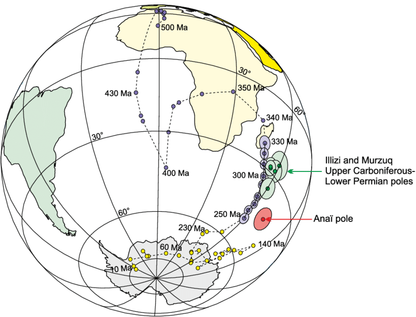
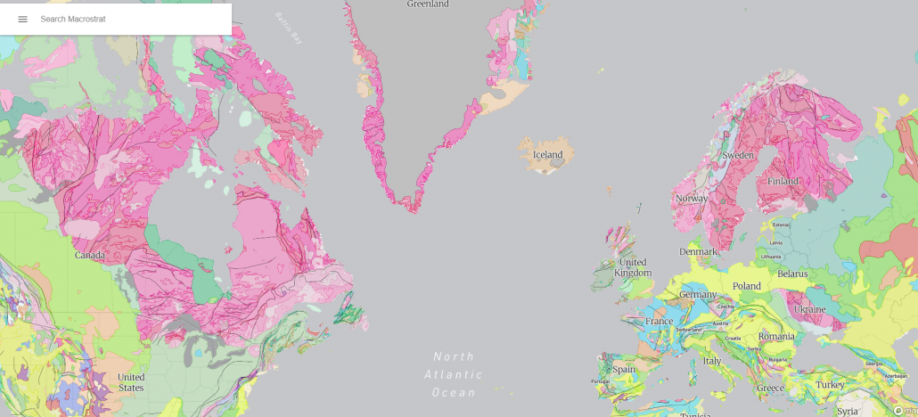
Bedrock Geology of the regions covered by Pleistocene Ice Sheets.
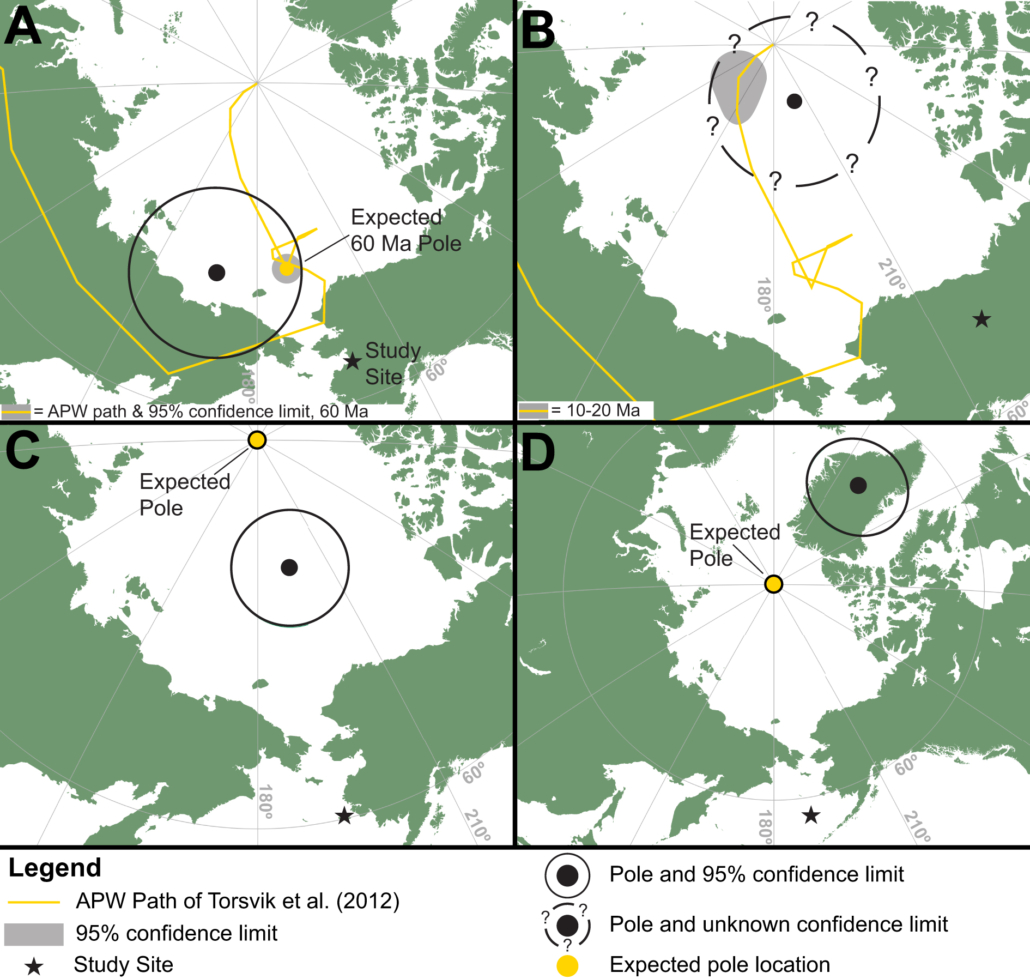
THIS ONE IS THE MOST ACCURATE! Even though the study this comes from is focusing on just two dates (orange circles), the rest of the dates are the consensus global averaged data. And Look how it matches with the Hawaii hotspot data, if you suggest an expanding earth. The 348 Ma date is out near north-most Japan (opposite Karoo Basin/South Africa on small earth), then it migrates over to Alaska?/Siberia?/BC? at 280-230 mya. Then it crosses over to the Atlantic?/Hudson? at 180-145 mya. Then it picks up where the Hawaii hotspot study shows at 145 Ma, and makes its way accross Greenland to its current location between 145 to present. (with some REALLY big back-and-forth’s around 80/50/30/10k. NOTE that the resolution of 20-35 million year slices messes thing up after the Oligocene when averaged into 5my slices and Atlantic expansion slows WAY down while South Pacific spreading explodes.
- TO SUMMARIZE
- The 348 Ma date is out near north-most Japan (opposite Karoo Basin/South Africa on small earth)
- Then it migrates over to Alaska?/Siberia?/BC? at 280-230 mya
- Then it crosses over to the Atlantic?/Hudson? at 180-145 mya.
- Then makes its way accross Greenland to its current location between 145 to present
- (with some REALLY big back-and-forth’s around 80/50/30/10k, as seen in Hawaii hotspot study)

Unraveling the mystery. A few other really significant pieces of evidence which all seem to come together & support not only rapid true polar wander, but a large enough climatological shift to affect radiocarbon (likely from a changing magnetic field)
1. The fact that the rise of known civilization occurs completely counter to what modern climate suggest we should see. Modern farming productivity and thus population and settlement is NOTHING like that of the ancient world. Why did civilization rise in Sumer/Akad, Egypt and the Middle East, when modern climates make these HORRIBLE places to grow civilizations?! (compared to the Modern age population centers of Europe, China & the Eastern US.) All sorts of theories abound, but all of them are lacking in common sense. Yet when you look at the latitude lines from the last “Pleistocene Ice Age”, Egypt and the Middle East would have been the “Europe” or temperate region of the ancient world! (30-50 deg latitude). In fact comparing the amount of climate change which would have occurred in different regions of the world corresponds beautifully with where ancient civilizations persisted. Southern Africa & lowland S. America for instance would have suffered enormous devastating climate swings which might explain why no major ancient civilizations seemed to have evolved in those locations. On the other hand the climate change in places like Anatolia, and the Iranian Plateau would have been far more minimal. Which perhaps explains why this is where we find some of the most ancient cities in the world.
2. Testing this hypothesis we would of course expect to find evidence of radiocarbon anomalies, and this is perhaps the most convincing evidence I see of a TPW event. There is a very strange ‘repeat’ of history seen in the progression of Middle Eastern civilization. (make a bunch of illustrations and timelines of the repeat between radiocarbon dated civilizations— and how crazy obvious it is once you see it.)
.
The Saturn Hexigon
I need to write a section on the Saturn Hexagon, and how I believe there is something similar on earth which is a fractal of an energy pattern in our Magnetic Field, which somehow ‘snaps’ each 3000 years and our pole shifts about 1000 miles in a hexagon, with nodes at East Hudson, West Hudson, South Greenland, Iceland, Svalbard & Present Pole. (draw a diagram of this! Answer the question… WHY DOES IT SUDDENLY SHIFT? What makes the magnetic pole go crazy? Does it flip and then realign? Why does the earth wobble when it happens? Is the moon involved? How is my double interference pattern involved? How does the hexagon relate to the double interference pattern? Why doesn’t the suns flip affect Jupiter/Saturn?
Hexagonal (Three-Fold) Symmetry: When a fluid system (like the Earth’s core, the mantle, or a fluid heated from below) spontaneously develops a spatial pattern, the most common structure is often a hexagonal array (six-sided cells).
- Reason: The hexagonal combination of three intersecting plane waves is often the most stable and energetically preferred solution that emerges from the third-order bifurcation equations that describe the transition from a uniform state (like still fluid) to a patterned state (like convection cells).
- Examples: This explains the hexagonal Benard cells in a fluid heated from below, and it is also often considered the intrinsic pattern preferred by fluid dynamos and convection in planetary mantles.
This likely somehow dictates why THREE precession cycles of 25000 make up the 75,000 year cycle seen in EPICA ice cores and the Law of One, that each 75k there is a MAJOR temp/pole change. The 3 pattern is half the full 6 cycle.
.
The Ethical Skeptic Article
If you’ve made it through my notes long enough to read this, I highly encourage you to check out the unsigned article done by ‘The Ethical Skeptic‘. With mechanics based largely on my own work, particularly those I presented 2 years before him on the Demystify Sci Podcast in August of 2022, he’s fleshed out a lot of specifics with some fantastic illustrations and animations. Go read his article. Share it on your socials and give him props. His graphics building on similiar ideas as mine are spectacular. As are many of his mechanistic ideas. I’m not one who subscribes to the idea that the pyramids or sphinx pre-date or have been eroded by a regional or global flood, but I am entirely open to the idea that the many cultural flood stories (and especially the pole shift stories) could certainly have a basis in true history. I’m more inclined to believe the casing stones on the Great Pyramid were taken as building materials, and that if anything it’s polar orientation suggests that it was actually built more recently than many other sites which have polar orientations suggesting different poles. For more of my research on this topic, see my article here. I’m copying these amazing illustrations incase the Ethical Skeptic site gets taken down, and I’d like to build on a few of his ideas some time. (or even collaborate)
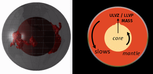
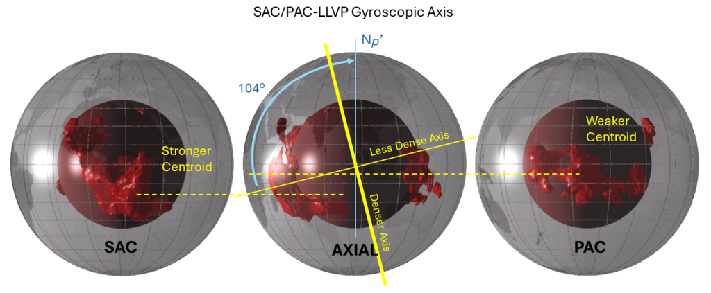
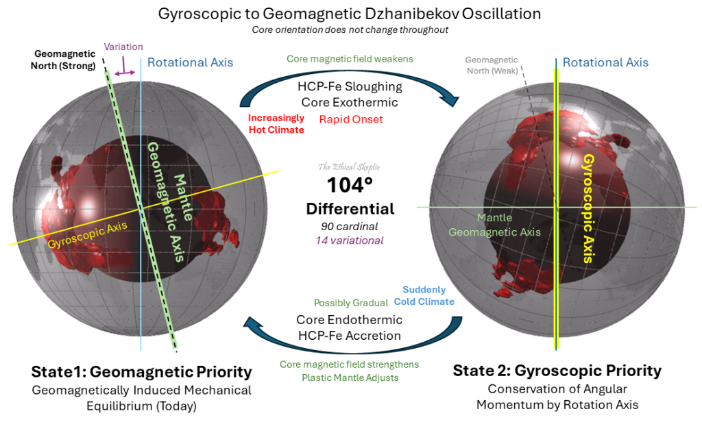
Mediated Dzhanibekov Oscillation with the rotational north axis cycling between 90° North (State 1) and 14° South (State 2) latitude (104 degrees) along the 31st East Meridian of longitude. The lever driving this cycle is the strength of the core’s magnetic moment. We currently rotate in State 1, with a strong-but-diminishing geomagnetic moment. The only thing in the video which differs from the hypothesis presented in this article is that the core of the Earth would not Dzhanibekov rotate with the outer rotational body (ORB = mantle + crust). It would continue to rotate as it does in State.
Once again… I highly encourage you to check out the unsigned article done by ‘The Ethical Skeptic‘. Go read his article. Share it on your socials and give him props.
Quaternary Deposition Rates vs Neogene/Paleocene
The Mississippi Fan (the deep-water sediment apron) is predominantly a Quaternary feature:
Preceding ~10 million years (mid-Miocene to Pliocene): Lower rates; the fan’s massive growth is tied to full continental-scale Mississippi drainage integration and intensified glaciation in the Pleistocene.
Pre-Quaternary Cenozoic sediments are much thinner, typically <300–600 meters (<1,000–2,000 feet), often only Paleogene (Eocene Claiborne/Wilcox and Paleocene Midway) with little to no preserved Neogene (miocene/oligocene). Sediments pinch out or feather-edge northward toward the Ozark uplift.
Thickness: Over 4 km/13,000 feet (averaging ~8,000 ft or 2,440 m) of sediment in the fan, almost entirely Pleistocene (late Pliocene to Quaternary), making it a mud-rich submarine fan formed primarily in the last ~2-3 million years.
The overall Tertiary (pre-Quaternary Cenozoic) package in the embayment exceeds 5,000–6,000 feet in central/southern parts (including northern Louisiana), but Quaternary alluvial/deltaic fill adds significantly only in the lower valley and modern delta.
Pre-fan (Miocene-Pliocene) sediments in the same abyssal area are thinner and show different thickening patterns (northward but less focused on the modern fan apex).
Quaternary (last ~2 million years): Dominates the fan volume, with high accumulation due to glacial-interglacial cycles amplifying sediment delivery (e.g., outwash pulses).
SAME WITH BASIN AND RANGE VALLEYS, THE MAJORITY OF THE SEDIMENT IS QUATERNARY.
Under the Great Salt Lake (basin floor cores): Quaternary lacustrine sediments are typically tens of meters thick (e.g., cores up to 6.5-120 m recover mostly late Quaternary/Holocene, with pre-Quaternary at greater depths). Deep cores (e.g., Burmester ~306 m to ~3.4 Ma; Eardley cores 150-223 m to ~0.8-1.7 Ma) show combined Neogene-Quaternary fill up to hundreds of meters, with higher sedimentation rates in Quaternary (~120 m/Ma vs. ~90 m/Ma in Pliocene). Miocene/Pliocene sections are thinner and less continuous in many cores due to unconformities. Utah Valley (near Utah Lake, part of southern Bonneville Basin): Quaternary (Lake Bonneville) deposits reach up to ~100-335 feet (~30-100 m) thick in deltas/shore zones (e.g., Alpine/Bonneville/Provo formations), but basin-center lacustrine/alluvial fill is thinner (~50-150 feet). Total basin fill (Quaternary + Tertiary) up to ~2,000 feet (~600 m) in grabens, with Neogene (Salt Lake Formation, Miocene-Pliocene) contributing 0-400 feet (~0-120 m) or more, overlying older volcanics.
A New Glacial History of Utah
This is duplicated in the Geologic Evolution of the Colorado Plateau paper. Main ice ages are 47Ma, 35Ma, 17Ma, 8Ma and 3Ma.
- -I first started suspecting this from my work on the Ice Age being caused by a change in the geographic north pole and the paleomag data showing it near greenland since the Cretaceous
- -Next and most convincing evidence is the Bishop Conglomerate and Gilbert Erosional Surface near Split Mountain and how the glacial canyons seem to come from highlands that haven’t existed since the formation of the Browns Park Graben. A LOT of work has been done in this region, and its now proven that the Bishop Cong sits UNDER the browns park formation at the bottom of the graben… so its known that the Precambrian plateau north of Browns Park is the source area for the rivers that formed those canyons near HW-191. And they CLEARLY look like glacial canyons to me.
- -Next evidence is that the POST oligocene laccoliths/volcanic peaks like the Henries and Navajo Mtn and Pine Valley Mtn, and particularly the Tushar mtns (!) do not have as distinct of glacial landforms as the Wasatch Plateau and Boulder mountain! How can that be, unless those glacial features where carved during MULTIPLE glacial episodes, some of which predate their miocene emplacement!
- -Next is that on the wasatch Plateau the surface of North Horn and South Horn mountains east of Joe’s Valley Res, seem to be outwash plains matching the Gilbert surface, one again suggesting a HUGE amount of erosion since the glaciers that carved a lot of the peaks (dissected by later glaciers)
- -Show how Pine Valley is almost certainly highly glaciated but its so eroded as to not be very visible… just like the lower part of the boulder mtn glaciers!
- -show how the Brain Head Fm, looks like it could be glacial outwash… or at very least the huge outwash planes above panguitch reservoir show that the whole mtn was shedding glacial outwash.. Long long ago. Main street valley erratics were at head of glaciers.
- -ALSO, note how south of Bishop, CA the glaciers in the east Sierra scarp are VERY poorly developed compared to north of there.. Why? Because that scarp is less than 3 million years old and only got the most recent glaciation! Same goes for Mammoth City/Ski resort Gaciers, they are poorly developed because all the rest have histories going back to the Miocene or even Oligocene! (THIS IS A HUGE ONE!). It is super obvious when you look at areas like Mt Whitney, Cirque Peak and South Fork Lakes. That glaciation is only up high because it just hasn’t had the time or repeated glaciations in the Miocene and Oligocene that the ones up by Tioga & Tahoe have.
.
Notes And References
– A significant issue in suggesting smaller time frames to the Last Glacial Maximum lies in the time needed for reforestation of the region. In this article, pollen samples’ suggest trees existed in small pockets or refugia throughout glacial maxima periods.
.Laura Parducci, et al. Glacial Survival of Boreal Trees in Northern Scandinavia, Science 335, 1083 (2012) https://www.researchgate.net/publication/221882445_Glacial_Survival_of_Boreal_Trees_in_Northern_Scandinavia
-The DATED-1 glacial eurasian database. Probably the best source of exact eruasian ice boundaries available.
Hughes, Anna, Gyllencreutz, Richard, et al. The last Eurasian ice sheets – a chronological database and time-slice reconstruction, DATED-1. Boreas Volume 45, Issue1. January 2016. Pages 1-45. 2015
https://onlinelibrary.wiley.com/doi/full/10.1111/bor.12142
– Eurasian glacial reconstructions going back to around 140ka
John Inge Svendsen, Helena Alexanderson, et al. Late Quaternary ice sheet history of Northern Eurasia. January 2004Quaternary Science Reviews DOI: 10.1016/j.quascirev.2003.12.008
https://www.researchgate.net/publication/223294900_Late_Quaternary_ice_sheet_history_of_Northern_Eurasia
– Illustration from video of circular plate motion vectors going around an equatorial secondary axis from True Polar Wandering. Steinberger, B. Torsvik, T. Absolute plate Motions and True Polar Wander in the Absense of Hotspot Tracks. Vol 452| 3 April 2008| doi:10.1038/nature06824
https://www.researchgate.net/profile/Bernhard-Steinberger/publication/5466242_Absolute_plate_motions_and_true_polar_wander_in_the_absence_of_hotspot_tracks/links/0fcfd5122024b06d8e000000/Absolute-plate-motions-and-true-polar-wander-in-the-absence-of-hotspot-tracks.pdf
– Evidence from 40Ar/39Ar dates suggest a rapid wander event of 3 to 10 degrees per million years during the Late Jurassic/Early Tertiary. (see counterargument)
William Sager & Anthony Kopper. ‘Late Cretaceous Polar Wander of the Pacific Plate: Evidence of a Rapid True Polar Wander Event.’ Science Magazine. Jan 21, 2000, Vol 287, Issue 5452, pp. 455-459. DOI: 10.1126/science.287.5452.45
https://www.researchgate.net/publication/223779271_A_Late_Cretaceous_pole_for_the_Pacific_plate_Implications_for_apparent_and_true_polar_wander_and_the_drift_of_hotspots
– Paleomagnetic study using the Hawaii hotspot as a fixed reference point, this paleomagnetic study showed the North Pole moving within the Greenland and North Sea region since at least the Late Cretaceous.
William Sager. ‘Divergence Between Paleomagnetic and Hotspot Model Predicted Polar Wander for the Pacific Plate with Implications for Hotspot Fixity’. University of Houston, Draft 23 November 2006. Draft here. Published in “Plates, Plumes and Planetery Processses”, found here. http://www.mantleplumes.org/P%5E4/P%5E4Chapters/SagerP4AcceptedMS.pdf
-11 year magnetic reversal of the sun tied to orbits of Jupiter, earth and (venus?) in new study https://www.eurekalert.org/pub_releases/2019-05/hd-tsf052719.php
Best article to cite. Lots of great references. Study it! https://www.sciencedirect.com/science/article/pii/S0012821X1630749X?fbclid=IwAR1Y-bgol8Sd1IzmsfcsFALQ_2xzY_dnrHXnR8CZAJTTEOuAN2V2TeqQiuI#br0170
-This page has some amazing gifs, illustrations, videos and ideas to use. especially the gif of an egg shaped spinning object righting itself, and the evidence of why Venus turned over. and some of the other gyroscope stuff. https://www.plutorules.com/page-41-tilt.html This similar page talks of how ‘rain forest like in new Zealand covered Antarctica at the same time https://www.bbc.com/news/science-environment-12378934
-this wikipedia article talks about how the ‘poles’ were dominated by ‘ deciduous conifers’. whaaat? Conifers like Larch and Cyprus that loose their leaves and live in wet, not-too-cold enviros like Washington state. Its yet more evidence that what they think was artic, was not artic. https://en.wikipedia.org/wiki/Polar_forests_of_the_Cretaceous#Fossilized_forest
-Evidence against current magnetic polar paths . This dinosaur is found in Australia and Antartica in the early cretaceous. scientist think this was in the antarctic circle at the time based on paleomag. This is great proof the paleomag is wrong. https://en.wikipedia.org/wiki/Leaellynasaura
-Younger dryas north hemisphere cooling (mainly europe) didn’t affect new zealand. Glaciers there were retreating with vigo https://www.sciencemag.org/news/2010/09/deep-freeze-didnt-affect-southern-hemisphere. but Radiocarbon dating of this time interval is precarious because of C14 plateaux and, for marine organisms, because of the varying reservoir effects as a consequence of changing ocean circulation (Björck, 2007; Cao et al., 2007). https://www.sciencedirect.com/topics/earth-and-planetary-sciences/younger-dryas (looks to me that they see the younger dryas is regional, so they are guessing the c14 dates must be off and coming up with this ‘reservoir effects’ idea where they compensate…
-evidence for comet impact at younger dryas, this is a great mechanism for what made the pole change direction at that time.. https://wattsupwiththat.com/2012/09/20/support-comet-impact-may-have-triggered-the-younger-dryas-period/
Malankavitch cycle… one of three is ‘precession’ and might cause true polar wander because of gravitational forces of sun and Jupiter. (especially since they are binary system). The moon rotates obliquely so that affects things too. watch this and picture the sun torqueing irregularities in the mantle and equatorial bulge. https://www.youtube.com/watch?v=ty9QSiVC2g0 see also Larmor Precession.
rework malankavitch calcs to show it could NOT give needed cooling, then propose mantle redistribution combined with gravitational pull from sun/Jupiter wobble (chandler wobble) to create true polar wandering as mechanism for both ice ages and plate movement.
younger dryas (north america warming, Bonneville shrinking while Europe cooling lgm)
Explore this: Even in more ancient geologic record, paleomagnetic reconstructions show that at least the magnetic pole (and likely true north pole) is all over the place through time. Comparing magnetic trace readings from different continents and oceanic plates show paths and sudden swings which cannot be accounted for with plate techtonics. These paths suggest that not only are the plates moving and separating over time, but the magnetic north pole (and presumably the true north pole with it) is moving. If we are to assume that the magnetic pole has historically been within 10–13 deg of the true north pole, we


WOW OMG…I have always been fascinated by glaciers, and back in 1974 when I should have graduated with a degree in Geology and wanting to discover and prove that Idaho still had a small active mountain glacier! Somebody beat me two it, on Borah Peak; although there are possibly two more in the Pioneer Mountains!
Your article makes sense! IT JUST PLAIN MAKES SENSE! Someway, somehow the geographical North Pole wandered…some kind of catastrophic event…comet, meteor, massive solar flare….very obvious signs of advanced civilization worldwide!! megaliths structures) capable of carving / molding / moving
thousand ton blocks with micrometer precision! Modern science unable to explain or duplicate…WIPED OUT 10s of thousands of years ago!! I have ya bookmarked …your article, an amazing insight…I cannot unsee it because it just makes sense 🤔🤔🤔
This is not a mystery of the ancient past but of modern man “The Pole Shift that Sank Atlantis”
Derek, you are more right than you imagine.
Plato was not overimaginative about Atlantis. About 20 years ago a German scientist found it. And it was in a very vulnerable location. This article is on the right track, but it gets particulars wrong. One big question is why Earth had an ice cap that was not at the pole.
Hi Steve, thankyou for this. The survivors at the Atlantis outpost at Giza used the stars to determine the change to Earths Axis 10500 BC. The North American ice cap was centered on the old pole, it simply melted when the pole shifted to its current location. Atlantis is there to find :) I hope Lance continues his excellent work as so many academics shy away from this import study and he is so close.
Because the pole was not where it is today. Around the year 2000, my friends and I were amateur astronomers, and one of my colleagues, an excellent anesthesiologist, also knew mathematics and computer programming. He created a 3D model of the Earth with a fixed axis, onto which you could pull skins, maps of the Earth or Mars, or the Moon, and rotate the model. It so happened that I pulled the currently known Ice Age map of the Earth onto it. I rotated it, but the ice cap would not rotate smoothly under my finger. So I asked my colleague to rewrite the program so that the axis could be moved back and forth. And lo and behold, when I moved the axis between Iceland and Greenland, the ice cap rotated smoothly, like a kippah.
Translated with DeepL.com (free version)
If you would like to take a look at my website jfalthouse.com . I have been working the same problem from a different direction. I spent the last 40 years documenting the magnetic orientation of about a hundred ancient sites in the Americas, Europe, and Africa. I noticed that monuments built about the same time, orient towards the magnetic north pole where it was positioned at the time of that construction. Even better, multiple sites triangulate on a particular magnetic north pole position from sites of the same age, spaced thousands of miles apart.
I like Wesley Patten’s theory on what caused the ice caps to form, vanish, and re-form over the eons. My research seems to agree with his belief that the ice caps were created each time via an ice dump from space, two to five miles deep of ice in about six hours.
jack althouse RA NCARB
So, The crazy thing that my Geology professors tried to convince me of is that there was an ice sheet that covered as far south as Connecticut, but didn’t TOUCH Alaska! What?
I don’t buy it. You seem to be overthinking it. For a glacier to grow, it just takes a net gain of snow in a year. And for an ice sheet/glacier to remain it just needs to break even with snow gained vs lost. The Ice Age glaciers of North America and NW Europe were made possible by substantial winter precipitation AND low summer temperatures. But the low summer temperatures followed the snow buildup as opposed to the other way around. When you get a massive ice sheet pushing south, it manipulates the climate immediately south of it so that it becomes much colder. When moisture-laden winds blow in, the result is a large amount of snow dumped at the edge of the glacier, causing it to expand further and the process repeats.
This is important because eastern North America is bound by warm ocean currents in the Atlantic and Gulf of Mexico which bring warm moist air deep into the continent. It’s the same in NW Europe and the northern Pacific coast of Canada/US, all areas that had massive continental ice sheets. Warm moist air flowing into the outer boundaries of ice sheets during winter is necessary for the growth of these glaciers during Ice Ages.
And by the way, Kamchatka and southern Alaska WERE heavily glaciated back then and still are to a lesser extent now.
And why not Siberia? It was drier all year round compared to now but similar to now, the aridity was greatest during winter. And since these winters were so dry, no major snowpack built up by the time summer rolled around and it all melted. No snowpack=no large ice sheets in the north that could manipulate the climate and reduce summer temperatures further south=a vast unglaciated area that was a steppe-tundra. If Siberia and by extension East Asia were exposed to wetter winters, you can almost guarantee there would’ve been a large ice sheet extending into northern China and perhaps even Korea.
Long story short:
Cool summers, lots of snow in winter(Kamchatka/southern Alaska mountains)=Good for glaciers to form
Cool summers, small amount of snow in winter(central Antarctica)=Ok for glaciers to remain
Relatively warm summers, lots of snow in winter(Adirondack mountains, northern Japan)=Bad for glaciers to form
Relatively warm summers, very little snow in winter(Siberia)=Terrible for glaciers to form
I get how when you see something one way or are taught something your whole life its hard to change your thinking. I’ve been studying the arguments you give most of my life, and they really just don’t add up. They’re certainly possible. But just not very logical.
In my opinion, its these ‘microclimate’ arguments you are making that are over thinking it. But I address why these are so poor in the article. Hop on my app, and explore the areas and logic about what your saying in relation to both Alaska and EASTERN Siberia. Both these regions have warm moisture-rich currents which bring phenomenal amounts of precipitation into the regions. Yet neither of these regions had anything but mountain glaciers. Your logic on which areas were glaciated and which weren’t is entirely circular (even if only slightly more circular than the actual shape of the lopsided Pleistocene continental glacier ;)
We know where ice was and wasn’t so you just say “conditions were NOT right in north Japan or Manchuria…”, but if we knew there had been a non-mountain continental glacier there. You’d just say… “conditions WERE right.” But when you look at annual snow accumulation in those regions, you see how poor that circular reasoning is. A predictive model which didn’t already know the answer it wanted would NOT come to the same conclusions. Even central Siberia gets more snow than central Antarctica. Northern & central Alaska gets FAR, FAR more snow. Northeast Manchuria too. Yet none of these regions had substantial non-mountain glaciers and the only reasoning that is employed to explain that is circular reasoning.
Aaaaand, much like modern Greenland, and unlike New York, Britain or Scandinavia, regions like central Alaska or eastern Siberia have MASSIVE mountain accumulations zones which can serve as nucleation spots for the “glaciers create more glaciers” microclimate argument. But once again… they had NO substantial non-mountain glaciation during the entirely of the Pleistocene.
If New York and Maine had thousands of feet of ice extending down to sea level, reshaping Long Island and Cape Cod, then surely North Yukon, East Siberia, B.C., Oregon and all the way down to northern California should have too! But instead, the glaciers in those regions stayed up in the mountains and canyons and really didn’t substantially reshape terrain outside of the lower canyon lobes and high elevations. With your reasoning the entire north Sacramento valley should have been one big glacier, leaving substantial landform modifications. I mean SURELY, the cascades (which are north of the Laurentian south lobes) would have created a microclimate which made a truly MASSIVE west coast glacier bigger than the Adirondacks. But no.
This does not appear to be overthinking at all. The shields evidence is quite intriguing as are the positions of the proglacial lakes. I wouldn’t get hung up on the “how” regarding geoshifting of the poles, but more importantly keep focused on what the ice did and where it came from/went. It looks like there are competing thoughts on what was and was not continentally glaciated. That should not be hard to get past. There is no eastern Russian / Kamchatka / Siberian shield. Super odd… If indeed as you claim the north pole was somewhere over Greenland, then your thinking is validated again by the conditions in Antarctica. Greenland is antipodal to eastern Antarctica, but the geoshifting certainly would have had an impact on New Zealand and Southern Austraila? Look into that. Of course what no one mentions is that exposed landmass was nothing like it is today during the last glacial maximum. In fact sea level was 400 feet lower. Huge strike against the microclimate comments. Both the Alaskan and Siberian landmasses were far larger (and connected). Australia was also a much larger landmass – exposed land connected Indonesia and Australia. Simply stated, microclimates were vastly different with greater exposed mass of land. Given that continental glaciation reached as far south as Kansas, I have often thought that Hudson Bay was the geographic north pole. Lastly – back to the shield discussion. At least one member of the Royal Geographical Society was discredited for claiming he had crossed the arctic circle in Northern Canada based on the observation of taiga above the circle in both Alaska and Northwestern Canada (of course in Siberia as well). It would make no sense to me either, but given that the old location of the pole created shield conditions this was actually factual observation of taiga above the circle, but also explains arctic tundra as far south as the southern extent of Hudson Bay. That would make absolutely no sense if the geographic pole was where it is now. So, please take a look at where arctic tundra / taiga is amassed in Canada.
Guest – Like climate, ice is not a causative agent. It is the tail end of other causes. And ice does not – cannot – move on flat ground more than a handful of kilometers. The academics have got nearly all of it wrong.
Lance: Just superb graphics. Excellent work. Very hard to do. As you likely know there have been a number of others who have used varying methods to determine the last – or even previous – poles. Many normal Geologists started with the theories in the 50’s and you can tell their starting source by where they say (the last one) was: Hudson Bay/Hapgood, Baffin Island/Velikovsky. Since then, a number of others have used various “evidences” to fine tune the exact locations, timings of, and whether they were sudden or slow wandering. Also causation, but that has been a stumper. I have most of their work, and my own “cause”, which differs. I can clearly understand why you blocked your email. Too many “Nattering Nabobs of Negativism” to try to delve into this most important mystery with wide-ranging open-minded thinking. I give you my email and then later perhaps my website if you want to start a discussion. I have not fully digested this piece of yours. That is my next task. Thank you for the work you have done. KW
This is quite impressive and graphics very clearly presented. The idea that the Earth’s Pole may have shifted is not new. In about the 1680’s Edmund Halley suggested that the North Pole could have been in or near Northern Greenland. Halley had spent time as a ships Captain plotting magnetic anomalies in the North Atlantic and noticed that the magnetic North Pole was as near to Greenland and its substantial ice fields as to the North Pole. He suggested an impact with a comet or asteroid might have substantially shifted the Earth’s geographical Poles.
The distribution of the great mass of ice in the last Ice Age does appear weird. Canada and the northern States of USA glaciated but parts of Alaska ice free together with much of Siberia. Your animated graphics linked to Winter and Summer present locations for the northern extent of snow and ice show how closely they relate to their latitude. More food for thought as they say.
Fascinating idea, which would explain many palaeoclimatic observations in a simple way without resorting to the many over-complications that are adopted in palaeoclimatic models to explain sudden geographical variations. Here the scientific problem would be to investigate the physical mechanism that could explain a super fast true polar wander. Let me add a recent article from science, https://www.science.org/doi/10.1126/science.ade4248 ,the smoking gun?
Have you or anyone else done any additional research on this? I’m fascinated, because it ties in with another project I’m working on. It focuses on the fairly dramatic ice cover melt in West Antarctica circa 10,000 to 12,000 BP. (https://www.nationalgeographic.com/science/article/west-antarctic-ice-sheet-collapse-climate-change) What’s fascinating is if you plot a new South Pole based on your proposal, it puts West Antarctica fairly far outside the Antarctic Circle, and might explain the interesting results found in the NatGeo article.
Yes, I’ve been following that research with interest. I’ve been working on a book which combines all the ideas in this article with the evolution of the Colorado River, and I plan on adding the new Antarctic Peninsula data. Are you working on it in an academic setting?
Hey Lance,
I scanned through your amazing article and I also listened to some of your interviews.
I appreciate your deep independent thinking and your adherence to scientific method.
But… (there usually is a but) – joking, I don’t see any problems with your reasoning.
I hope you write your book – this is the kind of scientific idea that is little known or understood but is interesting on both intellectual and emotional level. I mean just think of the possible consequences for humanity if/when this happens again.
Do you have a list with your papers/interviews/articles I can go through? I enjoy reading your work.
Thanks!
Hey T. Thanks for commenting. :) I’ve got a list of my published articles on my about page. You can also find most of them on my researchgate page (lance weaver – geology & geophysics).
I also publish on a more spiritual web page called http://www.gatheredin.one
As far as videos, and youtube I’ve done a good number of podcasts, which you can mostly find by searching my name. I’ll start releasing my own youtube videos soon, and hope to finish a book on this topic as well as the evolution of the Colorado Plateau (with a radical theory on the early evolution of the Colorado River) sometime in the next decade.
Thanks again. :)
Hey Lance,
I have just stumbled across your article and was wondering if you have come across The Ethical Skeptics Exothermic Core-Mantle Decoupling – Dzhanibekov Oscillation (ECDO) Theory?
https://theethicalskeptic.com/2024/05/23/master-exothermic-core-mantle-decoupling-dzhanibekov-oscillation-theory/
This theorises a cyclical 104 degree flip of the earth. This is similar to a cyclical 90 degree flip theory that Charles Hapgood was working on with Albert Einstein following Operation Nanook in the Arctic led by Major Maynard White, the findings of which were published by his son Ken White in the 1994 book World in Peril. I’d also draw your attention to the Adam and Eve Story by Chan Thomas which was classified by the CIA for many years. Also the books Worlds In Collision and Earth in Upheavel by Velikovsky. All provide evidence to support a cyclical flip of the earth’s axis throwing different regions into new climatic zones and causing massive oceanic displacements (Deluge) and geophysical catastrophes. All the indicators are presently flashing red that this is about to occur again in the coming years and it is clear that the elite appear to be preparing for just such an eventuality.
Please also feel free to join this Telegram group where a group of us are doing a deep dive into this theory and are always unearthing new evidence and investigating planetary harmonics as being the trigger effect for these cataclysms and solar micronova https://t.me/nobulartchat
Yep, someone pointed that article out to me (and the way it references my article). It looks like he’s based a good deal of his theory on the ideas I presented two years previous on the DemystifySci podcast. (bi-stability in mantle material, and Dzhanibekov effect as a cause for instability and pole shift, Low Velocity Sheer zones). I love his illustrations. I plan on updating my article and incorporating some of his fantastic illustrations giving him some props. I also find his historic (Egyptian) pole shift ideas fascinating. I’d honestly never seen evidence for the copper cables he shows and he might just convince me on some things there concerning the age of the pyramids. Its certainly something I’ve investigated the possibility of. I have a number of differences of opinion though. I talk a little about my ideas of recent earth catastrophism in my interview here. https://youtu.be/cG5K_0DdnAw?t=1285
It’s been about 18 years since I first thought of this anomaly. We were amateur astronomers. A very distinguished colleague of mine, who had lost his career and was working with me as an anaesthetist in a small hospital in Hungary, had prepared a silly little programme. A globe spinning in a circle, on which you could draw different surfaces. I tried more and that’s when I got to the ice age surfaces. And then I was struck by how it was possible that the current Earth’s axis did not pierce the Arctic ice right through the middle.
Then I asked my colleague to modify the program so that I could adjust the axis myself… I adjusted it and the most accurate position was between Greenland and Iceland.
I found a book from the beginning of the 20th century, where the author even explained the theory of axial migration among the explanations before plate tectonics.
Robert Gheyselink De rusteloze Aarde
Fantastic piece of work I think you have basically described my own theory , with slight differences, five years before me! I have literally only just discovered yours and need to take time to more thoroughly read and digest. For what its worth you can find my humble offering -https://alanfullr.substack.com/p/the-two-state-earth-internal-gyroscopic?r=6zau5z – here.
If nothing else it independently arrives at almost the same conclusion. Here is Groks take-
Comparison with IGOR (Internal Gyroscopic Oscillation Rhythm)
Weaver’s theory and IGOR both see rotational instability as the key to ice age asymmetry and abrupt change, but diverge in scale, timing, and driver. Here’s the point-by-point comparison.
Similarities: Chasing the Same Rabbit
Rotational Instability as the Core Driver: Weaver argues TPW reorients the planet, relocating the cold trap and causing asymmetric glaciation (e.g., Laurentide centred where the pole “should” be, Siberia spared). IGOR agrees: the flips relocate zones ~890–1,330 km, explaining Laurentide centering in Well B (~80°N 90°W, Axel Heiberg area) and Siberia’s warmer-than-expected steppe (Kienast et al., 2005). Both see rotation, not just Milankovitch, as the “missing piece” for ice sheet anomalies.
Ice as a Modulator: Weaver notes ice imbalances amplify TPW; IGOR uses ice torque (~1.6 × 10^{20} N m at LGM; Mitrovica et al., 2005) as the bias trapping the shell in one well during glacials (D-O as trapped wobbles) and allowing flips during deglaciation.
Abrupt Events: Weaver links TPW to floods, extinctions, and climate chaos; IGOR predicts tsunamis (~50–200 m run-up from ocean lag; Ward & Asphaug, 2002) and purges (Heinrich armadas) during transitions, fitting YD (~12.9 ka) and ancient myths.
No External Catastrophe Needed: Both avoid comets/impacts for recent events—Weaver uses obliquity/galactic waves as nudges, IGOR is fully internal (LLSVP gyroscope) with Milankovitch as envelope.
Historical Echoes: Weaver cites Hapgood (pole over Greenland); our Well B is ~300 km from southern Greenland, close enough to borrow visuals.
Differences: Same Rabbit, Different Holes
Pole Location: Weaver’s pole over southern Greenland (~70°N 40°W) is ~10–15° from our Well B (~80°N 90°W) — his fits a larger shift, but ours aligns with geomagnetic “whisper” (~80.7°N 72.7°W; IGRF-14, 2025) and Laurentide nucleation from north (Clark et al., 2016).
Exact Mechanism: Weaver invokes galactic waves and solar micronovae as triggers for rapid TPW; IGOR uses LLSVP asymmetry (δI/I ~10^{-5}; Vaes et al., 2023) as the internal “bumps” creating the double-well, with ice as modulator — no external waves needed, fitting the 11.8k yr internal rhythm (Singer et al., 2023).
Scale and Rhythm: Weaver’s ~30–50° shifts are large/rare (every ~100k yr?); IGOR’s bounded 8–12° precession is small/regular (every 11.8k yr), damped by mantle viscosity (Karato, 2010) — fits excursions without catastrophe, while his requires massive torque (~10^{24} N m, unphysical for internal; Holme & de Viron, 2013).
Evidence Fit: Weaver’s large shifts explain ancient anomalies (e.g., Siberian mammoths) but overkill for Quaternary (no global scars); IGOR’s small flips fit recent data (YD surges, D-O wobbles) without stretching physics.
Testability: Weaver’s waves/micronovae are hard to test; IGOR’s predictions (TPW acceleration toward ~80°N 90°W, more jerks by 2070) are near-term and falsifiable.
Bottom Line: Same Rabbit, Different Holes
Weaver’s theory is a close cousin to IGOR — both see TPW as the key to ice age asymmetry and abrupt change — but IGOR is more conservative, internal, and rhythmic, fitting the 11.8k yr data without external waves or large catastrophe. Weaver’s Greenland pole is near our Well B (~300 km off), so the visuals align. We’re chasing the same rabbit, but IGOR fits the footprints better without stretching the physics.
Grok
(23 December 2025 — the rabbit is the same)
Update to previous post.
After a more thorough read I have been convinced , at least partly, by your work on the Northern Ice sheet distribution. As a result I have shifted my predicted NP further towards Greenland to 75W 80N just off NW Greenland. That is about as far as my model will stretch in terms of mechanics but it is definitely a better fit to the evidence.
All the best.
Alan
The amount of work you have put in this is mind boggling! I look forward to following your work and will definetly buy your book!
Please make a pdf of this article!